Use CVaR to capture tail risk


Use CVaR to capture tail risk
Use CVaR to capture tail risk
In today’s issue, I’m going to show you how to compute the conditional value at risk (CVaR) of a portfolio of stocks.
In a previous newsletter issue, you calculated the value at risk (VaR) of a portfolio. VaR estimates how much your portfolio might lose over a set time. One of the caveats with VaR is it assumes the distribution of returns is normal, which it’s not. Another caveat is VaR assumes losses will not exceed the cutoff point, which they likely will.
CVaR captures more information than VaR
CVaR is an improvement over VaR and is considered superior by practitioners. It takes into consideration the actual shape of the distribution and quantifies the tail risk. CVaR is also known as the expected shortfall since it measures the expectation of all the different possible losses greater than VaR.
Non-professional traders and investors should consider using CVaR over VaR for their own risk management. Unfortunately, most don’t.
By the end of this issue, you’ll know how to:
- Get stock data
- Compute VaR and CVaR
- Visualize the differences between the two
And do it all in Python.
Let’s go!
Step 1: Get stock data
Start by importing the libraries and getting the data. I like to use yfinance for getting stock data and NumPy for math functions. Soon, I’ll use the OpenBB SDK for data.
1import numpy as np
2import pandas as pd
3import yfinance as yf
4
5import matplotlib.pyplot as plt
import matplotlib.pyplot as plt
I’m going to use 90 stocks in the S&P 100 index. Grab the data and compute the returns.
1oex = ['MMM','T','ABBV','ABT','ACN','ALL','GOOGL','GOOG','MO','AMZN','AXP','AIG','AMGN','AAPL','BAC',
2       'BRK-B','BIIB','BLK','BA','BMY','CVS','COF','CAT','CVX','CSCO','C','KO','CL','CMCSA',
3       'COP','DHR','DUK','DD','EMC','EMR','EXC','XOM','META','FDX','F','GD','GE','GM','GILD',
4       'GS','HAL','HD','HON','INTC','IBM','JPM','JNJ','KMI','LLY','LMT','LOW','MA','MCD','MDT','MRK',
5       'MET','MSFT','MS','NKE','NEE','OXY','ORCL','PYPL','PEP','PFE','PM','PG','QCOM',
6       'SLB','SPG','SO','SBUX','TGT','TXN','BK','USB','UNP','UPS','UNH','VZ','V','WMT',
7       'WBA','DIS','WFC']
8
9num_stocks = len(oex)
10
11data = yf.download(oex, start='2014-01-01', end='2016-04-04')
12
13returns = data['Adj Close'].pct_change()
14returns = returns - returns.mean(skipna=True) # de-mean the returns
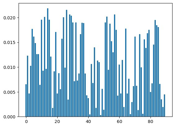
Create a mock portfolio by generating random weights and multiplying them by the returns. You can use your actual weights to represent your own portfolio.
1def scale(x):
2    return x / np.sum(np.abs(x))
3
4weights = scale(np.random.random(num_stocks))
5plt.bar(np.arange(num_stocks),weights)
Start by building a function to compute VaR so you can compare it to CVaR.
Step 2: Compute VaR and CVaR
Start by building a function to compute VaR so you can compare it to CVaR.
1def value_at_risk(
2    value_invested,
3    returns, weights,
4    alpha=0.95,
5    lookback_days=500
6):
7    returns = returns.fillna(0.0)
8    portfolio_returns = returns.iloc[-lookback_days:].dot(weights)
9
10    return np.percentile(portfolio_returns, 100 * (1-alpha)) * value_invested
First, replace any NaNs with 0.0s in the DataFrame of returns. Then take the last few days of returns and multiply them by the portfolio weights to create portfolio returns. Finally, compute VaR by taking the 5th percentile of returns and multiplying it by the value invested. This gets the amount you can expect to lose in one day with 95% confidence.
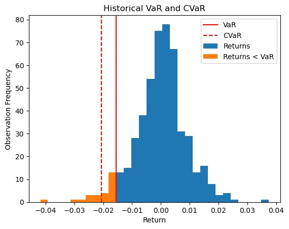
This is the main difference between VaR and CVaR. VaR represents a worst-case loss associated with a probability and a time horizon. CVaR is the expected loss if that worst-case threshold is crossed. In other words, CVaR quantifies the expected losses that occur beyond the VaR cutoff. VaR only measures the cutoff.
1def cvar(
2    value_invested,
3    returns,
4    weights,
5    alpha=0.95,
6    lookback_days=500
7):
8    var = value_at_risk(value_invested, returns, weights, alpha, lookback_days=lookback_days)
9
10    returns = returns.fillna(0.0)
11    portfolio_returns = returns.iloc[-lookback_days:].dot(weights)
12    var_pct_loss = var / value_invested
13
14    return np.nanmean(portfolio_returns[portfolio_returns < var_pct_loss]) * value_invested
Compute VaR to get the cutoff point on the distribution that equals the 5th percentile. Then compute the portfolio returns and convert VaR back to a percentage instead of a dollar amount. To compute CVaR, take the average of all returns less than VaR and multiply by the invested value.
Taking the average of all returns less than VaR is the same as taking the area of the distribution left of that cutoff point.
Step 3: Vizualize the difference between the two
Compute the CVaR and VaR of the portfolio and note the difference.
1cvar(value_invested, returns, weights)
2
3value_at_risk(value_invested, returns, weights)
CVaR is a bigger negative number than VaR. The difference between the two is the extra information CVaR captures by taking the average of all returns less than VaR. If you are dependent on VaR for risk management, you miss that information.
If this still isn’t clear, a chart will help.
1lookback_days = 500
2
3portfolio_returns = returns.fillna(0.0).iloc[-lookback_days:].dot(weights)
4
5portfolio_VaR = value_at_risk(value_invested, returns, weights)
6portfolio_VaR_return = portfolio_VaR / value_invested
7
8portfolio_CVaR = cvar(value_invested, returns, weights)
9portfolio_CVaR_return = portfolio_CVaR / value_invested
10
11plt.hist(portfolio_returns[portfolio_returns > portfolio_VaR_return], bins=20)
12plt.hist(portfolio_returns[portfolio_returns < portfolio_VaR_return], bins=10)
13plt.axvline(portfolio_VaR_return, color='red', linestyle='solid')
14plt.axvline(portfolio_CVaR_return, color='red', linestyle='dashed')
15plt.legend(['VaR', 'CVaR', 'Returns', 'Returns < VaR'])
16plt.title('Historical VaR and CVaR')
17plt.xlabel('Return')
18plt.ylabel('Observation Frequency')
Returns are not normally distributed. CVaR captures it.
Well, that's it for today. I hope you enjoyed it.
See you again next week.
