Manage your portfolio’s risk with value at risk

Manage your portfolio’s risk with value at risk

In today’s issue, I’m going to show you how to compute the value at risk (VaR) of a portfolio of stocks.

VaR is one way professional traders manage risk. It estimates how much your portfolio might lose over a set time period. Using VaR is a good way to avoid losing all your money if the market moves against you.

VaR lets you say something like this:

“With 95% confidence, my portfolio’s loss will not exceed $750 in one day.

Unfortunately, most non-professional traders don’t use VaR. They either don’t know it exists or think it’s too complicated to use.

I’m going to show you how to use Python to compute VaR using the variance-covariance method.

Let’s go!

Step 1: Import the libraries

We’ll use a new library today: scipy. Scipy is a library for scientific and technical computing. It has a lot of statistical functions.

I’m using Jupyter Notebook and want to plot my charts inline which is what %matplotlib inline does.

%matplotlib inline

import pandas as pd
import numpy as np
from scipy.stats import norm
import matplotlib.pyplot as plt

import yfinance as yf

Step 2: Define the variables

We’ll simulate a portfolio of stocks. To do this, we need to define the symbols, the weights, and the investment amount.

We also define the confidence level which we’ll use later.

# create your portfolio of stocks
tickers = ["AAPL", "FB", "C", "DIS"]

# pick the weights of each stock (must add to 1)
weights = np.array([0.25, 0.3, 0.15, 0.3])

# the size of the portfolio
portfolio_value = 1_000

# the confidence interval (95%)
confidence = 0.05

Now we can get the stock data for all the symbols in one line of code.

data = yf.download(tickers, start="2018-01-01", end="2021-12-31")["Close"]

Step 3: Compute portfolio statistics

Computing portfolio returns is not as simple as just adding up the returns of the individual stocks. We need to take the covariance between the stocks in the portfolio into account.

Fortunately, this is easy in Python using pandas and NumPy.

# compute daily returns of each stock
returns = data.pct_change()

# compute the daily mean returns of each stock
mean_returns = returns.mean()

# compute portfolio mean return
port_mean = mean_returns.dot(weights)

# mean of investment returns
investment_mean = (1 + port_mean) * portfolio_value

# compute the portfolio covariance matrix
cov_matrix = returns.cov()

# compute portfolio standard deviation
port_stdev = np.sqrt(weights.T.dot(cov_matrix).dot(weights))

# standard deviation of investment returns
investment_stdev = portfolio_value * port_stdev

First, we get the daily returns of the stocks in the portfolio. From there we get the mean return for all the data. We apply the weights to those returns and multiply them by the portfolio value to get the portfolio mean return.

Then we compute the covariance between the returns, take the square root of the covariance-adjusted weights of the stocks in the portfolio, and compute the portfolio standard deviation.

The portfolio mean and standard deviation are used in the next step.

Step 4: Compute VaR

To find the VaR of this portfolio, we start by finding the point on the density plot based on the confidence level, mean, and standard deviation.

This is where scipy comes in.

# ppf takes a percentage and returns a standard deviation 
# multiplier for what value that percentage occurs at.
# It is equivalent to a one-tail test on the density plot.
percent_point = norm.ppf(confidence, investment_mean, investment_stdev)

VaR is the portfolio value less this amount.

# calculate the VaR at the confidence interval
value_at_risk = portfolio_value - percent_point

# print it out
f"Portfolio VaR: {value_at_risk}"

This is the most you can expect to lose in one day with 95% confidence.

Bonus: Scaling VaR to different time frames

What about over one week? Or one month?

Stock returns increase with the square root of time. Therefore to scale the value at risk, we multiply it by the square root of time. This sounds scary but it’s simple in Python.

Multiply the one-day VaR by the square root of one (day) through the square root of 30 (days).

value_at_risks = value_at_risk * np.sqrt(range(1, 31))

Then we plot it.

# build plot of VaR over time
plt.xlabel("Day")
plt.ylabel("Max loss")
plt.title("Portfolio VaR")
plt.plot(value_at_risks, "r")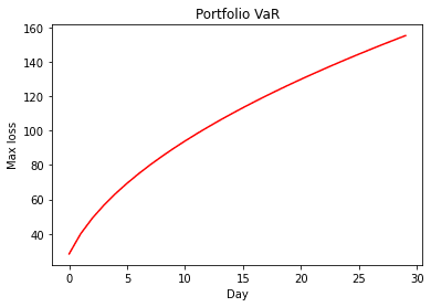

VaR is a simple measure that comes with various assumptions, caveats, and criticisms. It should be used as one of many risk management techniques. Despite its simplicity, it is a useful tool in the trader’s tool belt.

Read more about VaR here.