Value at risk (VaR) is a tool professional traders use to manage risk. It estimates how much a portfolio might lose, given normal market conditions, over a set time period.

There are three ways to compute VaR: the parametric method, the historical method, and the Monte Carlo method.

In contrast to the parametric and historical methods which are backward looking, Monte Carlo is forward looking.

In today’s newsletter, you’ll be able to simulate the equity curve of a portfolio of ETFs and compute the VaR using the Monte Carlo Method.

If you’re ready, let’s go!

Quickly compute Value at Risk with Monte Carlo

The Monte Carlo method for computing VaR involves generating a large number (sometimes millions) of hypothetical simulations of the evolution of a portfolio.

The scenarios correspond to a potential future value of a portfolio considering asset prices, weights, and covariances.

By simulating these scenarios, we can estimate the distribution of the portfolio’s future value.

From there, we can figure out VaR by identifying the worst losses at a specific confidence level, usually the 95th percentile.

The VaR represents the maximum amount of money we can expect to lose over a set time horizon.

Luckily for us, Python makes it easy to do.

Imports and set up

We only need three libraries for today’s issue. NumPy for the linear algebra, pandas for building DataFrames, and OpenBB for data. We’ll start by downloading data for a mock portfolio of 25 sector ETFs.

1import numpy as np
2import pandas as pd
3from openbb import obb
4
5sectors = [
6    "XLE", 
7    "XLF", 
8    "XLU", 
9    "XLI", 
10    "GDX", 
11    "XLK", 
12    "XLV", 
13    "XLY", 
14    "XLP", 
15    "XLB", 
16    "XOP", 
17    "IYR", 
18    "XHB", 
19    "ITB", 
20    "VNQ", 
21    "GDXJ", 
22    "IYE", 
23    "OIH", 
24    "XME", 
25    "XRT", 
26    "SMH", 
27    "IBB", 
28    "KBE", 
29    "KRE", 
30    "XTL", 
31]
32
33data = obb.equity.price.historical(
34    sectors, 
35    start_date="2022-01-01", 
36    provider="yfinance"
37).to_df()

Next, we’ll compute the historic mean returns, weights, and covariance matrix.

1data["returns"] = data.groupby("symbol").close.pct_change()
2
3portfolio_stats = data.groupby("symbol").agg(
4    daily_returns=("returns", "mean"),
5)
6
7portfolio_stats["weights"] = 1 / len(sectors)
8
9covariance_matrix = (
10    data
11    .pivot(
12        columns="symbol", 
13        values="returns"
14    )
15    .dropna()
16    .cov()
17)

In today’s example, we use a simple average of past returns to represent future expected returns. We also use a static, equal weighted portfolio. From our returns, we can use pandas to compute the covariance matrix between the sector historic returns. We’ll use the covariance matrix in the Monte Carlo to simulate the covariance between assets in the future price paths.

Set up the Monte Carlo simulation

Now that we have our historical returns and covariance matrix, we can generate the simulated price paths.

1simulations = 1_000
2days = len(data.index.unique())
3initial_capital = 100_000
4
5portfolio = np.zeros((days, simulations))
6
7historical_returns = np.full(
8    shape=(days, len(sectors)), 
9    fill_value=portfolio_stats.daily_returns
10)

We start by defining the number of simulations, the number of days, and the initial portfolio capital. We set up arrays to store the portfolio values and historical returns. Next, we run the simulation.

1L = np.linalg.cholesky(covariance_matrix)
2
3for i in range(0, simulations):
4    Z = np.random.normal(size=(days, len(sectors)))
5    daily_returns = historical_returns + np.dot(L, Z.T).T
6    portfolio[:, i] = (
7        np.cumprod(np.dot(daily_returns, portfolio_stats.weights) + 1) * initial_capital
8    )
9
10simulated_portfolio = pd.DataFrame(portfolio)

First, we calculate the Cholesky decomposition of the covariance matrix. Sounds complicated but all it does is generate correlated random variables. In the loop, we generate a normally distributed random variable and adjust it by the Cholesky factor to simulate daily returns.

These returns are then used to calculate our cumulative portfolio returns over the time period for each simulation. Finally, we use the NumPy array output to construct a pandas DataFrame.

Analyze the results

Now that we have our simulate results, we can compute VaR and conditional VaR.

1alpha = 5
2
3def montecarlo_var(alpha):
4    sim_val = simulated_portfolio.iloc[-1, :]
5    return np.percentile(sim_val, alpha)
6
7def conditional_var(alpha):
8    sim_val = simulated_portfolio.iloc[-1, :]
9    return sim_val[sim_val <= montecarlo_var(alpha)].mean()
10
11mc_var = montecarlo_var(alpha)
12cond_var = conditional_var(alpha)
13
14ax = simulated_portfolio.plot(lw=0.25, legend=False)
15ax.axhline(mc_var, lw=0.5, c="r")
16ax.axhline(cond_var, lw=0.5, c="g")

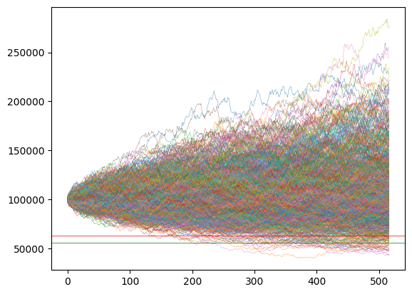
VaR is the value at the lower 5th percentile of the final portfolio values. It represents the dollar amount the portfolio will lose with 95% confidence.

The Conditional Value at Risk (CVaR) is also known as Expected Shortfall. CVaR is computed as the mean of the simulated values at the last time step that are less than or equal to VaR. Since CVaR captures the worst case losses beyond that of the point estimate provided by VaR, it’s often seen as a superior to VaR.

The plot visualizes all price paths, VaR, and CVaR. We can see that CVaR (the green line) is less than VaR which demonstrates the more conservative calculation.

Next steps

This simulation assumes static expected returns, no drift, no volatility, and a static covariance matrix. As a next step, use a look back window for the covariance matrix. You can also try introducing drift and volatility into the price paths.