Calibrating volatility smiles with SABR

In today’s newsletter, we’ll explore the SABR stochastic volatility model.

It’s a very popular volatility model used by professionals for many types of derivatives.

Today, we’ll look at how to calibrate the SABR parameters and use them to fit a volatility smile for equity options.

Sound good?

Let’s go!

Calibrating volatility smiles with SABR

The SABR model, built in 2002, stands as a key stochastic volatility framework in finance for modeling derivatives. SABR stands for “stochastic alpha, beta, rho” which are the key inputs to the model.

SABR is good at capturing the market-observed anomalies such as skew and smile.

It operates on the premise that asset prices follow a geometric Brownian motion while volatility follows an Ornstein-Uhlenbeck process, parameterized by alpha (initial volatility level), beta (variance elasticity), rho (price-volatility correlation), and nu (volatility’s volatility).

One of its standout features is the closed-form approximation for implied volatility—known as the Hagan formula—which allows for fast and accurate computations of implied volatility across strike prices.

Ready?!

Imports and set up

We’ll use the pysabr library to calibrate the SABR model, fit the volatility smile, and price options. Let’s import the libraries.

import pandas as pd
import numpy as np
import matplotlib.pyplot as plt
from openbb_terminal.sdk import openbb
from pysabr import Hagan2002LognormalSABR
from pysabr import hagan_2002_lognormal_sabr as sabr
from pysabr.black import lognormal_call

We’ll use OpenBB to fetch options prices for a ticker.

symbol = "SPY"
expiration = "2026-01-16"
spy = openbb.stocks.options.chains(symbol, source="YahooFinance")

From here, we’ll grab the calls and puts at the specified expiration.

calls = spy[spy.optionType == "call"]
jan_2026_c = calls[calls.expiration == expiration].set_index("strike")
jan_2026_c["mid"] = (jan_2026_c.bid + jan_2026_c.ask) / 2

puts = spy[spy.optionType == "put"]
jan_2026_p = puts[puts.expiration == expiration].set_index("strike")
jan_2026_p["mid"] = (jan_2026_p.bid + jan_2026_p.ask) / 2

strikes = jan_2026_c.index
vols = jan_2026_c.impliedVolatility * 100

We filter the DataFrame for call and put options at the given expiration. We then compute the mid price to get a more accurate picture of implied volatility. We’ll need the strikes and market implied volatilities, too.

Fit the SABR model

First, we compute the forward stock price using put-call parity, set the expiration, and assign a beta.

f = (
    (jan_2026_c.mid - jan_2026_p.mid)
    .dropna()
    .abs()
    .sort_values()
    .index[0]
)
t = (pd.Timestamp(expiration) - pd.Timestamp.now()).days / 365
beta = 0.5

Put-call parity defines the relationship between put options, call options, and the forward price of the underlying. You can read more here. The t parameter is the fraction of time until expiration.

The beta parameter governs the shape of the forward rate, which influences the shape of the implied volatility smile. A beta of 1 implies a lognormal distribution, which is consistent with the Black-Scholes model. Moving beta away from 1 allows for different shapes of volatility smiles. In practice, setting beta to 0.5 is usually a safe bet.

Once we set the parameters, we instantiate the model and call fit to get alpha, rho, and volvol.

sabr_lognormal = Hagan2002LognormalSABR(
    f=f,
    t=t,
    beta=beta
)

alpha, rho, volvol = sabr_lognormal.fit(strikes, vols)

The fit method calibrates the SABR model parameters to best fit a given volatility smile. The alpha parameter is a measure of the at-the-money volatility level, rho represents the correlation between the asset price and its volatility, and volvol which is the volatility of volatility.

Generate a fitted volatility smile

Now that we have alpha, rho, and volvol, we can generate the calibrated volatility smile.

calibrated_vols = [
    sabr.lognormal_vol(strike, f, t, alpha, beta, rho, volvol) * 100
    for strike in strikes
]

This code generates a lognormal volatility for each strike in our options chain.

Let’s plot it.

plt.plot(
    strikes, 
    calibrated_vols
)

plt.xlabel("Strike")
plt.ylabel("Volatility")
plt.title("Volatility Smile")
plt.plot(strikes, vols)
plt.show()

The result is a fitted volatility smile (or smirk in this case), along with the market based volatility smile.

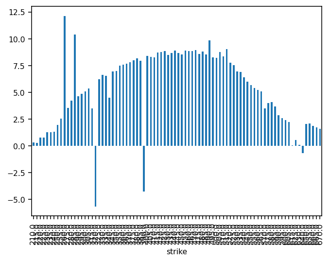
We can assess the model error as well.

black_values = []
for strike, calibrated_vol in zip(strikes.tolist(), calibrated_vols):
    black_value = lognormal_call(
        strike, 
        f, 
        t, 
        calibrated_vol / 100, 
        0.05, 
        cp="call"
    )
    black_values.append(black_value)

option_values = pd.DataFrame(
    {
        "black": black_values,
        "market": jan_2026_c.mid
    },
    index=strikes
)

(option_values.black - option_values.market).plot.bar()

The result is a bar chart which demonstrates the model error for each strike price based on the calibrated implied volatility from the SABR model.

Next steps

We breezed over a lot of the theory behind the SABR model. As a next step, take a look at the Wikipedia article on the SABR model. It will help get more intuition behind what’s happening.