Use Markov models to detect regime changes

It’s rumored that Renaissance Technologies uses hidden Markov models in their trading.

In fact, the Baum-Welch algorithm used with Markov models was partially invented by Leonard Baum who would help found RenTec.

In today’s newsletter, we’ll look an example of using a Markov model to detect regime changes in the equities market.

Let’s go!

Use Markov models to detect regime changes

A Hidden Markov Model (HMM) is a probabilistic model where a sequence of observable variables are generated by a sequence of hidden states. The important thing to note is the hidden states are not observed directly.

The observed variables can be things like price while the hidden states can be a market regime.

The transitions between hidden states assume to have the form of a Markov chain. They can be specified by the start probability and a transition matrix.

The emission probability of an observable variable can be any distribution based on the hidden state.

Let’s see how it works in Python.

Set up and imports

We’ll use the excellent hmmlearn library to fit our Markov model.

import numpy as np
import pandas as pd
import yfinance as yf
from hmmlearn import hmm

Next, import data for your favorite asset and compute our two features.

data = yf.download("SPY")
returns = np.log(data.Close / data.Close.shift(1))
range = (data.High - data.Low)
features = pd.concat([returns, range], axis=1).dropna()
features.columns = ["returns", "range"]

We’ll attempt to predict the unobservable market regime based on daily log returns and the day’s range.

Now let’s fit the model.

Fit the Markov model

Fitting the model is just a few lines of code.

model = hmm.GaussianHMM(
    n_components=3,
    covariance_type="full",
    n_iter=1000,
)
model.fit(features)

We initialize a HMM with Gaussian emissions. This is a simplified assumption that the observations in the HMM follow a normal distribution.

We configure the model to have three hidden states, representing different market regimes such as up markets, flat markets, and down markets.

We set the covariance type to “full”, indicating that the covariance matrices of the Gaussian distributions associated with each state are fully parameterized. This means each state’s distribution has its own full covariance matrix which allows for correlations between different dimensions of the data.

Then, we train the model on the features. During training, we iteratively adjust the model’s parameters over 1000 iterations to maximize the likelihood of the observed features given the hidden states

This last step is the magic that learns the underlying patterns and transitions between market regimes.

Once the model is fit, we can use the trained model to predict the hidden states of the input features.

states = pd.Series(model.predict(features), index=data.index[1:])
states.name = "state"
states.hist()

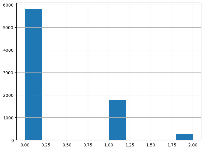
The predicted states are returned as a NumPy array which we use to create a pandas Series. The result is a histogram showing the number of daily states across the data.

Visualize the regimes

Finally, we can plot the price data colored by each of the various states.

color_map = {
    0.0: "green",
    1.0: "orange",
    2.0: "red"
}
(
    pd.concat([data.Close, states], axis=1)
    .dropna()
    .set_index("state", append=True)
    .Close
    .unstack("state")
    .plot(color=color_map, figsize=[16, 12])
)

The result is the following plot.

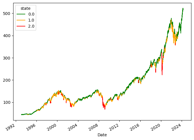
The model does a pretty good job detecting various market conditions, including upward trends (green), downward movements (red), and sideways markets (orange).

It’s important to note that the model’s assumption of a Gaussian distribution may not accurately capture the complexities of financial market data. As we know, the markets typically exhibit non-normal behavior.

Also note your output will look different since a HMM is a probabilistic model.

Next steps

To improve the model’s performance, you can try initializing it with customized transition probabilities and covariance matrices tailored to the features we use. You can also experiment with different emission probabilities, including Poisson distribution assumptions and custom models.