Active investing is hard. And if you can’t beat the benchmark, you might just want to buy the benchmark. When comparing performance, most people just look at returns which doesn’t capture the whole picture.

This is where tracking error comes in.

Tracking error measures how closely a portfolio follows its benchmark. It’s a great way to understand more deeply how your portfolio is performing.

By reading today’s newsletter, you’ll be able to use Python to compute and understand tracking error.

Let's go!

Use tracking error to test your investment skill

Tracking error quantifies the difference between a portfolio's returns and its benchmark. It’s a measure of how closely a portfolio follows its benchmark. A lower tracking error means the portfolio is closely tracking the benchmark. A higher tracking error means the opposite.

In practice, tracking error is calculated as the standard deviation of the differences between the portfolio's and benchmark's returns. It is used to evaluate performance and manage risk.

Professionals use tracking error to assess how well a portfolio manager replicates a benchmark. Index funds aim for low tracking error. That means they are efficiently replicating the benchmark. Actively managed funds accept higher tracking error for potential outperformance.

Let's see how it works with Python.

Import necessary libraries and generate sample data

We need to import the libraries and create a sample portfolio of sector-based ETFs.

1import numpy as np
2import pandas as pd
3import matplotlib.pyplot as plt
4import yfinance as yf
5import warnings
6warnings.filterwarnings("ignore")
7
8# Generate sample data
9symbols = [
10    "XLE",
11    "XLF",
12    "XLU",
13    "XLI",
14    "GDX",
15    "XLK",
16    "XLV",
17    "XLY",
18    "XLP",
19    "XLB",
20    "SPY"
21]
22data = yf.download(symbols, start="2020-01-01")["Adj Close"]
23returns = data.pct_change().dropna()
24benchmark_returns = returns.pop("SPY")
25portfolio_returns = returns.sum(axis=1)

We start by importing essential libraries: numpy for numerical operations and pandas for handling data structures. We then download price data for a series of sector ETFs which will serve as our portfolio. We include SPY as the benchmark. With the data, we can compute the portfolio and benchmark returns.

Calculate excess returns of the portfolio over the benchmark

We will now calculate the excess returns, which are the portfolio returns minus the benchmark returns.

1excess_returns = portfolio_returns - benchmark_returns

By subtracting the benchmark returns from the portfolio returns, we obtain the excess returns. This step helps isolate the portfolio's performance relative to the benchmark.

Compute the tracking error

We will compute the tracking error, which is the standard deviation of the excess returns.

1tracking_error = excess_returns.std()
2tracking_error

This measurement shows the volatility of the portfolio's performance relative to the benchmark. A higher tracking error indicates greater deviation from the benchmark, while a lower tracking error suggests the portfolio closely follows the benchmark. We use the std method to find the standard deviation of the excess returns.

Visualize the portfolio, benchmark, and excess returns

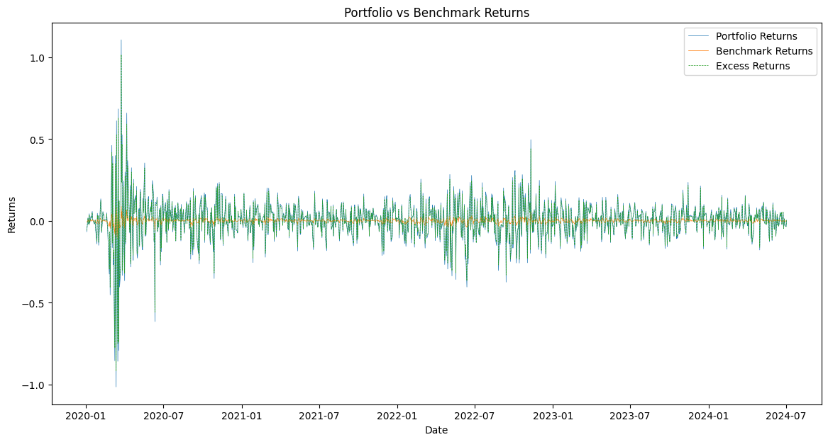
We will plot the portfolio returns, benchmark returns, and excess returns to visualize the performance.

1plt.figure(figsize=(14, 7))
2plt.plot(portfolio_returns.index, portfolio_returns, label='Portfolio Returns', lw=0.5)
3plt.plot(benchmark_returns.index, benchmark_returns, label='Benchmark Returns', lw=0.5)
4plt.plot(excess_returns.index, excess_returns, label='Excess Returns', linestyle='--', lw=0.5)
5plt.legend()
6plt.title('Portfolio vs Benchmark Returns')
7plt.xlabel('Date')
8plt.ylabel('Returns')
9plt.show()

We use matplotlib to visualize the performance of the portfolio, benchmark, and their excess returns. Plotting these values helps to see how the portfolio's returns compare to the benchmark over time. The plot function is used to create line plots for the portfolio returns, benchmark returns, and excess returns.

The result is a plot which shows the portfolio, benchmark, and excess returns.

Your next steps

This example uses ETFs to create a simple portfolio of one share each. Experiment with our own portfolio to see how it compares against the benchmark.