Understanding and managing the risk of ruin is a universal challenge for traders. I like to say that true risk management is about trading to live another day.

I've experienced the pain of watching capital evaporate because of poor risk management. (It’s one of the reasons I became a risk quant!) Most investors use diversification to manage risk and active traders use stop-loss orders.

Neither measures the risk of catastrophe, however.

I have always looked volatility as the de factor measure of risk. That’s because the more your equity curve moves around, the higher the risk of having to liquidate assets at a loss. Of course no single metric paints the whole picture.

And risk of ruin is an important perspective.

By reading today's newsletter, you'll get Python code to simulate a trading strategy and compute the risk of ruin.

Let’s go!

The risk of ruin is your scariest enemy (not just volatility)

The risk of ruin is the probability of losing enough capital to stop trading or investing. It is crucial for investors to understand this risk. The math is pretty easy and considers factors like initial capital, win/loss ratio, and the probability of a winning and losing trade.

In practice, risk of ruin is calculated using various models, including the Kelly Criterion and leveraging Monte Carlo simulations.

Professionals use strategies like diversification, position sizing, and stop-loss orders to mitigate the risk of ruin.

Some people make it complicated, but it doesn’t have to be.

Let’s see how it works with Python.

Imports and set up

All we need for this analysis is NumPy and Matplotlib. Import them first.

1import numpy as np
2import matplotlib.pyplot as plt

Define functions to simulate a trading strategy

First, create a simple function that simulates a trade result.

1def simulate_trade(win_prob, avg_win, avg_loss):
2    """
3    Simulate a single trade with given win probability and average win/loss amounts.
4    """
5    if np.random.rand() < win_prob:
6        return avg_win
7    else:
8        return -avg_loss

The simulate_trade function simulates the outcome of a single trade based on the win probability. If a random number is less than the win probability, the trade is a win, otherwise, it's a loss. The function returns the gain or loss accordingly.

Next, set up a function that simulates a large number of trades.

1def simulate_trading_strategy(initial_capital, trades, win_prob, avg_win, avg_loss):
2    """
3    Simulate the entire trading strategy over a given number of trades.
4    """
5    capital = initial_capital
6    capital_history = [capital]
7
8    for _ in range(trades):
9        capital += simulate_trade(win_prob, avg_win, avg_loss)
10        capital_history.append(capital)
11
12    return capital_history

This code simulates the entire trading strategy over a specified number of trades. Starting with the initial capital, each trade's result is added to the capital.

Finally, we'll calculate the risk of ruin. This is the probability that the capital will drop to zero or below at any point during the trading period.

1def calculate_risk_of_ruin(initial_capital, trades, win_prob, avg_win, avg_loss, simulations=100):
2    """
3    Calculate the risk of ruin over a number of trading simulations.
4    """
5    ruin_count = 0
6
7    for _ in range(simulations):
8        capital_history = simulate_trading_strategy(initial_capital, trades, win_prob, avg_win, avg_loss)
9        if min(capital_history) <= 0:
10            ruin_count += 1
11
12    return ruin_count / simulations

Simulate the strategy to compute the risk of ruin

The initial parameters set the stage for our simulation. We define initial capital, win probability, and average win/loss amounts.

1initial_capital = 10000
2average_win = 110
3average_loss = 100
4trades = 1000

We can now calculate the risk of ruin by running multiple simulations of the strategy.

1risk_of_ruins = []
2steps = range(30, 60)
3for step in steps:
4    win_probability = step / 100
5    risk_of_ruin = calculate_risk_of_ruin(initial_capital, trades, win_probability, average_win, average_loss)
6    risk_of_ruins.append(risk_of_ruin)

We calculate the risk of ruin for a trading strategy across a range of win probabilities. It iterates through win probabilities from 30% to 59%, computes the risk of ruin for each probability  and stores the results.

This allows for the analysis of how varying the win probability affects the risk of ruin for the given trading strategy.

Plot the risk of ruin across the range of win probabilities.

1# Plot the capital history
2plt.figure(figsize=(10, 6))
3plt.plot(steps, risk_of_ruins, label='Risk of ruin')
4plt.xlabel('Probability of a winning trade')
5plt.ylabel('Risk of ruin')
6plt.grid(True)
7plt.show()

The result is the following chart.

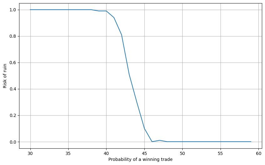
It should be no surprise that as the probability of a winning trade increases, the risk of ruin decreases. The key point here is that by increasing your average winner, you can reduce the risk of ruin despite a lower probability of a winning trade. It should also be apparent how import it is to quantify your results!

Your next steps

Change the average win/loss amounts to see how they affect the risk of ruin. Experiment with different initial capital values to understand their impact. To take it even further, feed your own trading results into the model. This will help you gain deeper insights into the robustness of various trading strategies.