I’ve taught 1,300+ how to build algorithmic trading strategies with Python.

I hear the same thing over and over:

Where do I start?

In my course, Getting Started With Python for Quant Finance, I teach the best way to start is with Minimum Viable Python.

Start with something simple, test, iterate, repeat.

That's where Pandas comes in.

With Pandas, you can quickly evaluate trading strategies using historical data to see if there’s evidence of an edge.

By reading today’s newsletter, you’ll learn how to assess a real trading strategy using Pandas.

Let's go!

Quickly test a profitable trading strategy (that actually works)

Fund managers report their holdings every month. They don’t want to tell investors they lost money on meme stocks. So at the end of the month, they sell low-quality assets and buy high-quality assets, like bonds.

We might be able to take advantage of this by buying bonds at the end of the month and selling them at the beginning of the month.

Why does this work?

The edge is probably too messy, too small, or just not interesting to professionals. Which makes it perfect for us.

Most people over-complicate algorithmic trading - it really can be this simple.

Here’s how to investigate this effect with Python, step by step.

Imports and set up

We’ll use yFinance for market data and of course pandas, then we download historical data for TLT, a long-term treasury bond ETF.

1import pandas as pd
2import numpy as np
3import yfinance as yf
4
5
6tlt = yf.download("TLT", start="2002-01-01", end="2024-06-30")
7tlt["log_return"] = np.log(tlt["Adj Close"] / tlt["Adj Close"].shift(1))

This code fetches the adjusted closing prices for TLT from Yahoo Finance. It then calculates the log returns, which provide a continuous compounding measure of the rate of return.

Log returns are useful because they are symmetric and additive over time.

The shift(1) function aligns the prices for the current and previous day to compute the return. This creates a new column in our DataFrame to store log returns for each trading day.

Analyze TLT returns by calendar day of the month

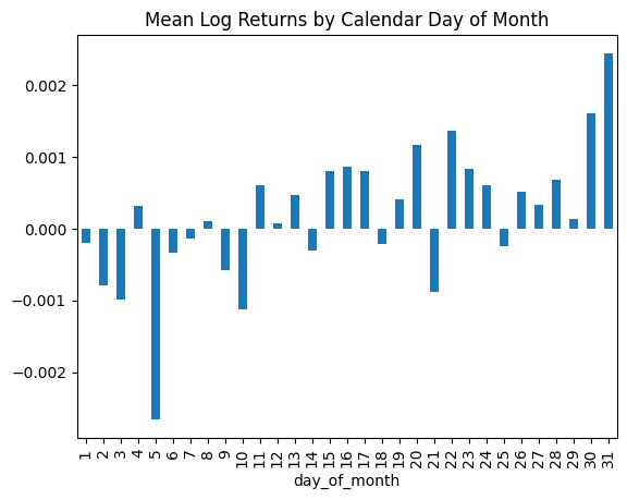
We add the day of the month and year to the data. This allows us to categorize and analyze the returns based on specific days. We then compute the average log return for each day of the month and visualize it with a bar plot.

1tlt["day_of_month"] = tlt.index.day
2tlt["year"] = tlt.index.year
3grouped_by_day = tlt.groupby("day_of_month").log_return.mean()
4grouped_by_day.plot.bar(title="Mean Log Returns by Calendar Day of Month")

The code extracts the day and year from the date index and adds them as new columns. It groups the data by the day of the month to calculate the mean log return for each day. This aggregation helps identify patterns or anomalies in returns on specific days.

We use a bar plot to visualize these average returns, making it easier to spot trends or outliers.

We expect there to be positive returns in TLT toward the end of the month. We expect this because we think fund managers buy TLT at the end of the month. We expect there to be negative returns in TLT toward the beginning of the month.

This is when fund managers sell their high-quality assets and go back to buying meme stocks.

We see evidence that returns are positive during the last days of the month and negative during the first.

Compare returns from the first and last week of each month

We create two new columns to store returns for the first and last week of each month. We then calculate the difference between these two to analyze how returns change from the beginning to the end of the month.

1tlt["first_week_returns"] = 0.0
2tlt.loc[tlt.day_of_month <= 7, "first_week_returns"] = tlt[tlt.day_of_month <= 7].log_return
3
4tlt["last_week_returns"] = 0.0
5tlt.loc[tlt.day_of_month >= 23, "last_week_returns"] = tlt[tlt.day_of_month >= 23].log_return
6
7tlt["last_week_less_first_week"] = tlt.last_week_returns - tlt.first_week_returns

This section initializes two new columns to zero to store returns for specific weeks. It assigns log returns to first_week_returns for days 1 through 7 and to last_week_returns for days 23 through the end of the month. We calculate a new column last_week_less_first_week to find the difference between these two periods.

This difference helps evaluate whether there are systematic return patterns between the start and end of the month.

Visualize yearly and cumulative strategy returns

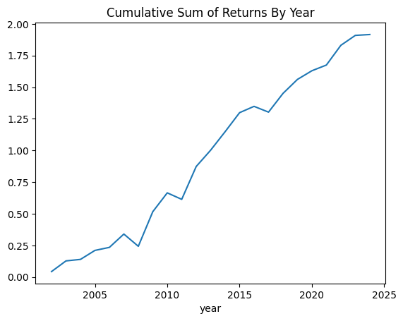
We analyze the strategy returns over time to understand the overall performance of the strategy.

1(
2    tlt.groupby("year")
3    .last_week_less_first_week.sum()
4    .cumsum()
5    .plot(title="Cumulative Sum of Returns By Year")
6)

The result is a plot of the annual returns. It looks like the strategy doubled the portfolio value.

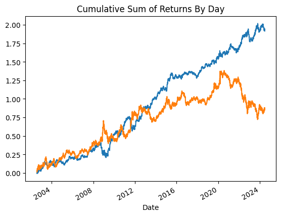
Now we can compare the strategy results to a buy-and-hold strategy.

1tlt.last_week_less_first_week.cumsum().plot(title="Cumulative Sum of Returns By Day")
2tlt.log_return.cumsum().plot()

Here, we plot the strategy results (blue) with TLT’s cumulative returns.

Our strategy outperformed the buy-and-hold strategy by almost double.

Your next steps

This is the Minimum Viable Python you need to assess a trading strategy.

Try altering the code to analyze a different asset or time period. You can change the ticker symbol or the date range to see how returns differ. Experiment with different months to check for seasonal patterns.