This is the first in many newsletters where I will cover RAPIDS, a suite of GPU-accelerated data science and AI libraries from Nvidia. These libraries have APIs that match popular open-source data tools like pandas and Polars.

RAPIDS is a suite of libraries that makes it easy to use accelerated computing with familiar tools like pandas and Polars. It unlocks the speed of GPUs with code you already know.

Part of the problem with pandas is that it can be slow with large data sets.

That’s where cuDF-pandas comes in. cuDF-pandas acclerates pandas with zero code changes and brings great speed improvements.

In today’s newsletter, you’ll get code to conduct mean-variance optimization on one-minute data using cuDF.

Using it, we’ll see a 9X performance speed up over pandas on CPUs.

(Make sure you check out your next steps at the end of this newsletter for a no-code change method of acceleration!)

Let’s go!

Portfolio optimization 9X faster with RAPIDS

RAPIDS works by leveraging GPUs' parallel processing capabilities.

It includes libraries like cuDF-pandas for data manipulation and cuML for machine learning, speeding up data science tasks. This accelerates risk calculations, optimizations, and machine learning applications in portfolio management.

Professionals in finance use RAPIDS for data processing, real-time analytics, and advanced optimization. Financial institutions report faster simulations and enhanced risk assessments. Robo-advisors have improved computational efficiency, crafting more personalized investment strategies.

Let's see how it works with Python.

Imports and set up

In addition to cuDF, we’ll use CuPy which is a GPU-accelerated array library. To work with this example, you can download the data here.

1import time
2import numpy as np
3import pandas as pd
4import cudf
5import cupy as cp

Now let’s build some helper functions.

Load and preprocess price data using pandas

First, we define a function to load our price data from a CSV file using pandas. The function will read the data, set the date as the index, and ensure all date indices are in the correct datetime format.

1def get_prices_as_pandas(prices_file):
2    d = pd.read_csv(prices_file)
3    d.set_index("date_time", inplace=True)
4    d.index = pd.to_datetime(d.index)
5    return d.bfill().ffill()

Next, we define a similar function to load the price data using cuDF, a GPU-accelerated library similar to pandas. This will allow us to perform computations on the GPU.

1def get_prices_as_cudf(prices_file):
2    c = cudf.read_csv(prices_file)
3    c.set_index("date_time", inplace=True)
4    c.index = cudf.to_datetime(c.index)
5    return c.bfill().ffill()

Note a few things. First, in the second function we use cudf.read_csv. Second, in both cases, w’ere backfilling and forward filling data. This means we’re copying prices into NaN values.

In practice, we’d be more careful about how we avoid sparse matrixes. But we’re showing the power of cuDF so in our case, it’s fine.

Compute optimal asset weights using pandas on the CPU

We will now compute the optimal asset weights using the classical Markowitz mean-variance optimization method with pandas. This involves reading the price data, calculating returns, and deriving the portfolio weights that minimize risk.

1print("=== Pandas (CPU) Computation ===")
2
3start_cpu = time.time()
4
5df_pandas = get_prices_as_pandas("intraday_prices.csv")
6n_assets = len(df_pandas.columns)
7
8df_returns_cpu = df_pandas.pct_change().dropna()
9mean_returns_cpu = df_returns_cpu.mean()
10cov_matrix_cpu = df_returns_cpu.cov()
11
12inv_cov_cpu = np.linalg.inv(cov_matrix_cpu.values)
13ones_cpu = np.ones((n_assets, 1))
14w_cpu = inv_cov_cpu.dot(ones_cpu)
15w_cpu = w_cpu / (ones_cpu.T.dot(w_cpu))
16
17end_cpu = time.time()
18cpu_elapsed = end_cpu - start_cpu
19
20print(f"CPU elapsed time: {cpu_elapsed:.4f} seconds")
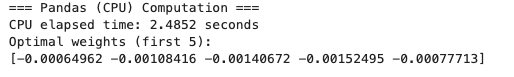
21print(f"Optimal weights (first 5):\n{w_cpu[:5].flatten()}")

We start by reading the price data and calculating daily asset returns as percentage changes. After computing the mean returns and covariance matrix, we use these to find the optimal portfolio weights that minimize variance.

The weights are computed using a closed-form solution involving the inverse of the covariance matrix. The elapsed time for these calculations is printed, along with the first few optimal weights.

The output will look something like this.

Perform the same computations using cuDF and cuPY on the GPU

Now, we will perform the same computations using cuDF and cuPY to leverage the GPU's computational power. This involves similar steps, but the operations will be accelerated by the GPU.

1print("=== cuDF (GPU) Computation ===")
2
3df_cudf = get_prices_as_cudf("intraday_prices.csv")
4n_assets = len(df_cudf.columns)
5
6start_gpu = time.time()
7
8df_returns_gpu = df_cudf.pct_change().dropna()
9mean_returns_gpu = df_returns_gpu.mean()
10cov_matrix_gpu = df_returns_gpu.cov()
11
12cov_cp = cov_matrix_gpu.values
13inv_cov_gpu = cp.linalg.inv(cov_cp)
14
15ones_gpu = cp.ones((n_assets, 1))
16w_gpu = inv_cov_gpu.dot(ones_gpu)
17w_gpu = w_gpu / (ones_gpu.T.dot(w_gpu))
18
19end_gpu = time.time()
20gpu_elapsed = end_gpu - start_gpu
21
22print(f"GPU elapsed time: {gpu_elapsed:.4f} seconds")
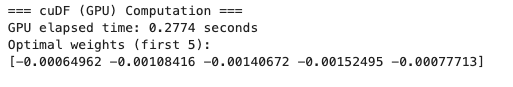
23print(f"Optimal weights (first 5):\n{w_gpu[:5].flatten()}")

This code performs similar operations as before, but using cuDF and cuPY. The GPU processes the same price data, calculating returns, mean returns, and the covariance matrix.

The covariance matrix inversion and weight calculations are accelerated by the GPU, resulting in potentially faster computations. We print the elapsed time and the first few optimal weights obtained through GPU processing.

The output will look something like this.

Finally let’s investigate the speed up.

Compare the computation times between CPU and GPU

We calculate the speedup achieved by using the GPU over the CPU. This comparison helps us understand the benefits of GPU acceleration for financial computations.

1speedup = cpu_elapsed / gpu_elapsed if gpu_elapsed > 0 else float('inf')
2print(f"Speedup (CPU / GPU) ~ {speedup:.2f}x")

You should see the speed up of using cuDF-pandas over pandas on CPUs. Running the code on my 2022 MacBook Pro M2 with remote access to an NVIDIA GPU, it’s ~9X faster with cuDF-pandas.

Your next steps

cuDF-pandas is available as an extension that requires no code changes at all. To use it, just add the following code before you import pandas.

1%load_ext cudf.pandas

That’s it!

With this method, you can enjoy the speed up using GPUs with the first version of code above. That means you can accelerate all your existing pandas-based notebooks with no code changes.

Give it a try!