Nobody can predict the future. But to price derivative securities like options, we must. Part of the problem is that asset prices often “jump.” Methods like Brownian Motion do not capture these jumps.

This is where the Poisson jump process comes in.

The Poisson jump process offers a more realistic way to model asset prices by including sudden jumps. Continuous models miss these jumps, which leads to inaccurate predictions.

By reading today’s newsletter, you’ll be able to use Python to simulate asset prices with Poisson jumps.

Let's go!

Poisson Jumps: Better pricing with a more realistic simulation

Simulating asset prices with Poisson jumps allows us to predict financial markets. The Poisson jump process incorporates drastic price changes that happen at random times. This model combines continuous price changes with sudden jumps. It can provide a more realistic representation of future prices.

In practice, the Poisson jump process uses a diffusion component for gradual price changes and a jump component for abrupt shifts. The diffusion is modeled using Brownian motion. The jumps are modeled using a Poisson process. This allows the model to capture real-world events like market crashes and rallies.

Financial professionals use the Poisson jump process in risk management, option pricing, and portfolio optimization. By including jumps, risk managers can better estimate risk metrics and create hedges. For option pricing, it can improve accuracy by capturing large price movements.

Let's see how it works with Python.

Import necessary libraries and define initial parameters

We will start by importing the necessary libraries and defining the initial parameters for the simulation.

1import numpy as np
2import matplotlib.pyplot as plt
3
4
5# Define parameters
6S0 = 100  # Initial stock price
7mu = 0.05  # Drift
8sigma = 0.2  # Volatility
9lambda_ = 0.1  # Jump intensity (average number of jumps per year)
10mu_j = -0.2  # Mean of the jump size
11sigma_j = 0.1  # Standard deviation of the jump size
12T = 1  # Time horizon (1 year)
13dt = 1/252  # Time step (1 trading day)
14N = int(T / dt)  # Number of steps

We are importing the required libraries: numpy for numerical operations and matplotlib.pyplot for plotting. We then define the initial stock price, drift, volatility, jump intensity, mean and standard deviation of jumps, time horizon, time step, and the number of steps for the simulation.

Simulate the asset price paths with Poisson jumps

Next, we will simulate the asset price paths considering both continuous returns and jumps.

1# Seed for reproducibility
2np.random.seed(42)
3
4# Initialize price array
5prices = np.zeros(N)
6prices[0] = S0
7
8# Simulate the asset price path
9for t in range(1, N):
10    # Generate the random components
11    Z = np.random.normal(0, 1)
12    J = np.random.normal(mu_j, sigma_j) if np.random.poisson(lambda_ * dt) > 0 else 0
13
14    # Calculate the price
15    prices[t] = prices[t-1] * np.exp((mu - 0.5 * sigma**2) * dt + sigma * np.sqrt(dt) * Z + J)

We use a fixed seed for reproducibility. We initialize an array to store the simulated prices and set the initial price. We then loop through each time step to simulate the asset price. Within the loop, we generate the normal random component for the continuous part and the jump component. We use Poisson distribution to decide if a jump occurs. The asset price is updated using the exponential model that includes drift, diffusion, and jump components.

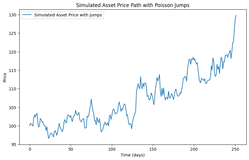
Plot the simulated asset price path

We will now visualize the simulated asset price path by plotting it.

1# Plot the simulated price path
2plt.figure(figsize=(10, 6))
3plt.plot(prices, label='Simulated Asset Price with Jumps')
4plt.xlabel('Time (days)')
5plt.ylabel('Price')
6plt.title('Simulated Asset Price Path with Poisson Jumps')
7plt.legend()
8plt.show()

We create a plot to visualize the simulated asset price path. We set the figure size, plot the prices, and label the axes. We add a title and a legend for clarity. Finally, we display the plot.

The result is a simulated price path which has visible jumps through time.

Your next steps

Now that you have simulated an asset price path with Poisson jumps, try changing some of the parameters. For example, adjust the jump intensity or the volatility to see how it affects the price path. Experiment with different time horizons or initial prices to gain a deeper understanding of the simulation.