In today’s newsletter, you’ll get a simple tool called the Tail ratio that helps with risk management.

There are many ways to compare two assets, and the Tail ratio can help inform your decision into which to buy or sell.

It works by comparing the extreme gains and losses in an asset or strategy. The more extreme gains, the higher the Tail ratio and vice versa.

By reading, you’ll get Python code to compute the Tail ratio between two assets.

Let’s go!

Performance made easy: The Tail Ratio for competitive analysis

Tail ratio is a unique tool in finance for evaluating extreme returns. It's a technique that compares high gains and steep losses. Tail ratio enhances visibility into economic shifts, particularly in volatile markets.

In practice, calculating the tail ratio involves arranging historical return data, determining return percentiles, and computing the 95th to 5th percentile ratio. This analysis assists in pinpointing the “tails” of gains and losses within strategies.

The best part is that it’s one line of code in Python.

Financial professionals use the tail ratio to assess hedge funds and for stress testing under extreme market conditions. The technique is crucial in determining risk-return balance and informs quantitative trading strategies.

Let's see how it works with Python.

Imports and set up

These libraries help us download financial data, analyze it, and create visualizations.

1import numpy as np
2import pandas as pd
3import matplotlib.pyplot as plt
4import yfinance as yf

We download stock data for NVDA and AMD, calculate daily returns, and prepare it for analysis.

1df = (
2    yf.download(["NVDA", "AMD"], start="2020-01-01")
3    .Close.pct_change(fill_method=None)
4    .dropna()
5)

This code fetches the closing prices for NVIDIA and AMD stocks from January 1, 2020, to the present. It then calculates the daily percentage returns and removes any rows with missing data.

The resulting DataFrame contains the daily returns for both stocks, which we'll use for our analysis.

Calculate the tail ratio

We define a function to compute the tail ratio and apply it to our stock data.

1def tail_ratio(returns):
2    return abs(np.percentile(returns, 95)) / abs(np.percentile(returns, 5))
3
4
5tail_ratio_a = tail_ratio(df.AMD)
6tail_ratio_b = tail_ratio(df.NVDA)
7
8print(f"Tail Ratio for AMD: {tail_ratio_a:.4f}")
9print(f"Tail Ratio for NVDA: {tail_ratio_b:.4f}")

The tail ratio is a measure of the relative size of the positive and negative tails of a distribution. Our function calculates this by dividing the absolute value of the 95th percentile by the absolute value of the 5th percentile.

We then apply this function to both AMD and NVIDIA returns and print the results. A higher tail ratio suggests more extreme positive returns relative to negative ones.

Visualize return distributions

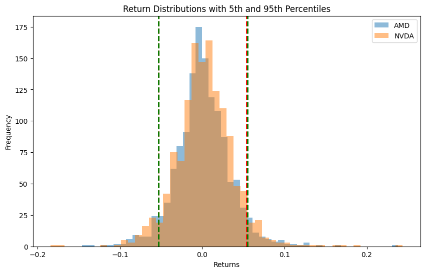
We create a histogram to compare the return distributions of AMD and NVIDIA.

1plt.figure(figsize=(10, 6))
2plt.hist(df.AMD, bins=50, alpha=0.5, label='AMD')
3plt.hist(df.NVDA, bins=50, alpha=0.5, label='NVDA')
4plt.axvline(np.percentile(df.AMD, 5), color='r', linestyle='dashed', linewidth=2)
5plt.axvline(np.percentile(df.AMD, 95), color='r', linestyle='dashed', linewidth=2)
6plt.axvline(np.percentile(df.NVDA, 5), color='g', linestyle='dashed', linewidth=2)
7plt.axvline(np.percentile(df.NVDA, 95), color='g', linestyle='dashed', linewidth=2)
8plt.legend()
9plt.title('Return Distributions with 5th and 95th Percentiles')
10plt.xlabel('Returns')
11plt.ylabel('Frequency')
12plt.show()

This visualization creates overlapping histograms of the daily returns for AMD and NVIDIA. We use 50 bins to show the distribution of returns for each stock. The 5th and 95th percentiles are marked with dashed lines for each stock.

This helps us visually compare the return distributions and see how the tail ratios we calculated earlier relate to the actual data.

Your next steps

The Tail Ratio is a simple tool to keep handy for comparing risk between two stocks. Given NVDA’s always in the news, it may seem like it vastly outperforms. In some ways maybe, but on a risk adjusted basis the performance is very similar as AMD. Test out the code with your favorite assets to see how they compare.