How to simulate stock prices with Python

In today’s issue, I’m going to show you how to simulate stock prices using Geometric Brownian Motion (GBM).

Simulating prices is fundamental for pricing derivatives. In the case of GBM, it is the key part of pricing equity options using Black-Scholes. Understanding how to simulate stock prices is foundational for any quantitative finance work. In fact, the math behind GBM was a good portion of my master’s degree.

The good news?

You don’t need a master’s degree to build your own stock price simulator in Python.

I’m going to show you how to do it.

Step by step.

But first: A quiz

Which stock price chart is real?

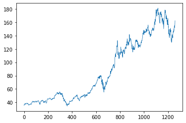
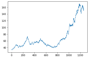
(Answer at the bottom.)

Step 1: What is Geometric Brownian Motion?

This is an abstract concept so I want to explain what GBM is all about.

Brownian motion comes from physics. It describes the random movement of particles in a substance. A Wiener process is a one-dimentional Brownian motion. It's named after Norbert Wiener who won a Nobel Prize studying one-dimentional Brownian motions.

The Wiener process features prominently in quantitative finance because of some useful mathemetical properties.

The GBM is a continuous-time stochastic process where where the log of the random variable follows the Wiener process with drift.

What?

It’s a data series that trends up or down through time with a defined level of volatility.

And it’s perfect for simulating stock prices.

Step 2: Import the libraries

I start by importing the libraries.

1import numpy as np
2import matplotlib.pyplot as plt

Since I’m simulating stock prices, I don’t need to download data.

Step 3: Set the input parameters

To simulate stock prices, we need some input parameters.

1# setup params for brownian motion
2s0 = 131.00
3sigma = 0.25
4mu = 0.35
5
6# setup the simulation
7paths = 1000
8delta = 1.0/252.0
9time = 252 * 5

Start by defining the initial stock price, s0. Then sigma which is the percentage volatility. Finally, mu (drift), which determine the overall trend.

Setup the simulation with 1,000 simulation paths. delta refers to the time step. I want to model a new stock price every day so I use 1/252 to represent 1 day in 252 trading days. The length of the simulation is 5 years.

Step 4: Build the functions

The first step is to build a function that returns a Wiener process. This function returns a 2-dimentional array with 1,260 rows and 1,000 columns. Each row is a day and each column is a simulation path.

1def wiener_process(delta, sigma, time, paths):
2    """Returns a Wiener process
3    
4    Parameters
5    ----------
6    delta : float
7        The increment to downsample sigma
8    sigma : float
9        Percentage volatility
10    time : int
11        Number of samples to create
12    paths : int
13        Number of price simulations to create
14    
15    Returns
16    -------
17    wiener_process : np.ndarray
18    
19    Notes
20    -----
21    This method returns a Wiener process. 
22    The Wiener process is also called Brownian 
23    motion. For more information about the 
24    Wiener process check out the Wikipedia 
25    page: http://en.wikipedia.org/wiki/Wiener_process
26    """
27
28    # return an array of samples from a normal distribution
29    return sigma * np.random.normal(loc=0, scale=np.sqrt(delta), size=(time, paths))

Next, I define a function that creates the GBM returns.

1def gbm_returns(delta, sigma, time, mu, paths):
2    """Returns from a Geometric brownian motion
3    
4    Parameters
5    ----------
6    delta : float
7        The increment to downsample sigma
8    sigma : float
9        Percentage volatility
10    time : int
11        Number of samples to create
12    mu : float
13        Percentage drift
14    paths : int
15        Number of price simulations to create
16    
17    Returns
18    -------
19    gbm_returns : np.ndarray
20    
21    Notes
22    -----
23    This method constructs random Geometric Brownian 
24    Motion (GBM).
25    """
26    process = wiener_process(delta, sigma, time, paths)
27    return np.exp(
28        process + (mu - sigma**2 / 2) * delta
29    )

Finally, I prepend a row of 1s to the returns array and multiply the starting stock price by the cumulative product of the GBM returns to produce the price paths.

1def gbm_levels(s0, delta, sigma, time, mu, paths):
2    """Returns price paths starting at s0
3    
4    Parameters
5    ----------
6    s0 : float
7        The starting stock price
8    delta : float
9        The increment to downsample sigma
10    sigma : float
11        Percentage volatility
12    time : int
13        Number of samples to create
14    mu : float
15        Percentage drift
16    paths : int
17        Number of price simulations to create
18    
19    Returns
20    -------
21    gbm_levels : np.ndarray
22    """
23    returns = gbm_returns(delta, sigma, time, mu, paths)
24
25    stacked = np.vstack([np.ones(paths), returns])
26    return s0 * stacked.cumprod(axis=0)

Step 4: Visualize the results

I want to demonstrate two examples.

The first example simulates 1,000 price paths over 5 years. It starts at a price of 131 with 25% annualized volatility and 35% average return per year. This is the volatility and return of Apple in 2021.

1price_paths = gbm_levels(s0, delta, sigma, time, mu, paths)
2plt.plot(price_paths, linewidth=0.25)
3plt.show()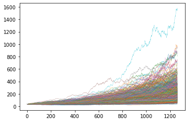

As you might expect, a 35% drift causes most price paths to increase from from the initial price. In fact we can test exactly how many have increased from the initial price.

1len(price_paths[-1, price_paths[-1, :] > s0])

999 of the 1,000 samples have increased.

In the second example I set the drift to 0.0.

1price_paths = gbm_levels(s0, delta, sigma, time, 0.0, paths)
2plt.plot(price_paths, linewidth=0.25)
3plt.show()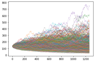

And I get a much different picture.

Only 402 prices end up higher than the original price.

Spend some time and play around with the variables. What happens if you double volatility? What happens if you set mu to a negative number?

Quiz answer: The first stock chart is AAPL. The second is a simulation.