How to compute drawdown on an investment

In today’s issue, I’m going to show you how to compute the drawdown of the SPY ETF with Python.

Drawdown is the maximum decline from peak to trough during a specific period before a new peak is reached. Every trading strategy experiences drawdowns. Computing it helps you compare the relative riskiness between assets or strategies.

Unfortunately, most people don’t consider drawdown when managing their investments. Or if they do, struggle to compute it.

Today I'm going to walk you through it step by step.

Step 1: Get the data

I start by importing the libraries I need.

1import yfinance as yf
2import numpy as np

Then I get data and compute the simple returns.

1data = yf.download("SPY", start="2020-01-01", end="2022-07-31")
2returns = data["Adj Close"].pct_change()

I use yfinance to get stock data – in this case, SPY. Drawdown is usually computed with the returns of a portfolio. I want to keep it simple so I use the S&P500 ETF.

Step 2: Create the drawdown function

Drawdown is computed with 4 lines of code.

When computing returns, the first value is turned into np.nan. I replace it with a 0.0 to compute cumulative returns. Then I create a cumulative return series which is the cumulative product of 1 plus the return. Next, I use NumPy's accumulate function. Accumulate tracks the running maximum value which is perfect for keeping tabs on the peak return.

Finally, I compute the percentage difference between the cumulative and peak returns.

Here’s the code:

1def drawdown(returns):
2    """Determines the drawdown
3    
4    Parameters
5    ----------
6    returns : pd.Series
7        Daily returns of an asset, noncumulative
8    
9    Returns
10    -------
11    drawdown : pd.Series
12    
13    """
14
15    # replace the first nan value with 0.0
16    returns.fillna(0.0, inplace=True)
17
18    # create cumulative returns
19    cumulative = (returns + 1).cumprod()
20
21    # np.maximum.accumulate takes the running max value
22    # of the input series. in this case, it will maintain
23    # the running maximum value. this is the running
24    # maximum return
25    running_max = np.maximum.accumulate(cumulative)
26
27    # compute the change between the cumulative return
28    # and the running maximum return
29    return (cumulative - running_max) / running_max

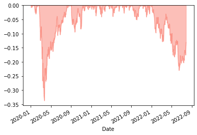
And the plot.

1drawdown(returns).plot(kind="area", color="salmon", alpha=0.5)

This chart shows SPY dropping 33.7% from its peak to trough return in 2020.

Step 3: Create a max drawdown function

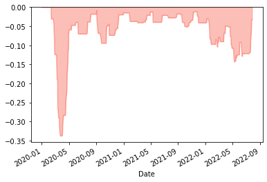
Next, I use the drawdown to compute a max drawdown chart.

The max drawdown differs from the drawdown by tracking the maximum drawdown of a 30-day rolling window of returns. To use rolling statistics, check out this issue of The PyQuant Newsletter.

Here’s the code.

1def max_drawdown(returns):
2    """ Determines the maximum drawdown
3    
4    Parameters
5    ----------
6    returns : pd.Series
7        Daily returns of an asset, noncumulative
8    
9    Returns
10    -------
11    max_drawdown : float
12    
13    """
14
15    return np.min(drawdown(returns))

max_drawdown applies the drawdown function to 30 days of returns and figures out the smallest (most negative) value that occurs over those 30 days. Then it moves forward one day, computes it again, until the end of the series.

Here’s the plot.

1returns.rolling(30).apply(max_drawdown).plot(kind="area", color="salmon", alpha=0.5)

Drawdown and max drawdown focus on capital preservation. It's a useful indicator of the riskiness of a stock, portfolio, or strategy. Use it to help manage your risk.