Managing risk is a key component to profitable investing.

Many traders use diversification to manage risk thinking it will shield them completely. Unfortunately, diversification can reduce unsystematic risk but leaves them vulnerable to systematic shocks.

In my early trading days, I thought diversification was the ultimate solution.

The Great Financial Crisis was a wake-up call when all correlations went to 1 and diversification no longer provided protection.

This pushed me to explore hedging techniques. Thankfully it’s easy in Python.

By reading today's newsletter, you'll be able to build a simple hedge to manage portfolio risk.

Let's go!

How to improve profits with a portfolio hedge

Investors face market risk, especially systematic risk, which affects entire markets.

Hedging is a strategy to manage this risk by reducing exposure to the benchmark. Professionals use sophisticated optimization techniques and derivatives to hedge. We can do it much more easily.

In a linear regression, beta measures the sensitivity of portfolio returns to the benchmark. For example, if your beta is 2.5, for every 1% decrease in the benchmark, the portfolio is expected to decrease 2.5%. When we construct portfolios, we want to isolate alpha (excess returns from skill).

To do it we hedge beta.

Let's see how it works with Python.

Imports and set up

We’ll only use two libraries for today’s analysis and download historical stock data for the Mag 7 mega cap tech stocks from Yahoo Finance. We will also calculate their daily returns to prepare for further analysis.

1import yfinance as yf
2import statsmodels.api as sm
3
4
5tickers = ['AAPL', 'MSFT', 'AMZN', 'NVDA', 'GOOG', 'META', 'TSLA', 'QQQ']
6data = yf.download(tickers, start='2022-01-01', end='2023-12-31')['Adj Close']
7
8benchmark_returns = (
9    data
10    .pop("QQQ")
11    .pct_change()
12    .dropna()
13)
14
15portfolio_returns = (
16    data
17    .pct_change()
18    .dropna()
19    .sum(axis=1)
20)
21
22portfolio_returns.plot()
23benchmark_returns.plot()

Using the yfinance library, we download the adjusted closing prices for our stocks.

We separate the returns of the benchmark ETF, QQQ, from the portfolio. We calculate the percentage change in adjusted closing prices for both the benchmark and the portfolio to get daily returns.

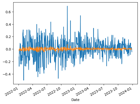
Finally, we visualize the daily returns of both our portfolio and the benchmark.

The blue line is our portfolio returns and the orange line is the benchmark. Our goal is to hedge out the benchmark returns.

Use OLS to perform regression and find hedge ratio

We will use linear regression to determine the relationship between our portfolio returns and the benchmark returns. This will allow us to understand how our portfolio is performing relative to the market.

1def linreg(x, y):    
2    x = sm.add_constant(x)
3    model = sm.OLS(y, x).fit()
4    return model
5
6X = benchmark_returns.values
7Y = portfolio_returns.values
8
9model = linreg(X, Y)
10alpha, beta = model.params[0], model.params[1]
11
12print(model.summary())
13print(f"Alpha: {alpha}")
14print(f"Beta: {beta}")

We define a function to perform linear regression using the statsmodels library. We add a constant to include an intercept (alpha) in the regression. This function returns a fitted model object that we can analyze.

We input the benchmark returns as the independent variable and the portfolio returns as the dependent variable. The regression provides us with an alpha and beta value. Alpha represents the excess returns of the portfolio not explained by the benchmark, while beta measures the sensitivity of the portfolio to market movements.

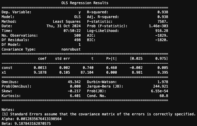
The summary of the model provides additional statistics to evaluate the fit.

The regression results indicate a very strong relationship between the portfolio and the benchmark, with an R-squared of 0.938. This means 93.8% of the portfolio's return variance is explained by benchmark movements.

The portfolio’s sensitivity to the benchmark is high, as shown by the coefficient of 9.19, suggesting amplified exposure. Unfortunately, our alpha coefficient is not statistically significant which implies there is little to no consistent excess return when the benchmark return is zero.

Implement the hedge using the calculated ratio

We will create a hedged portfolio by adjusting the portfolio returns based on the beta from our regression. We will then analyze the performance of this hedged portfolio.

1hedged_portfolio_returns = -beta * benchmark_returns + portfolio_returns
2
3P = hedged_portfolio_returns.values
4model = linreg(X, P)
5alpha, beta = model.params[0], model.params[1]
6
7print(f"Alpha: {alpha}")
8print(f"Beta: {round(beta, 6)}")

Using the beta from our previous regression, we adjust the portfolio returns to create a hedged portfolio. This involves subtracting the product of beta and benchmark returns from the portfolio returns, effectively reducing market exposure.

This is like saying “we’re short beta shares of QQQ and long the portfolio.”

We perform another regression analysis on the hedged returns against the benchmark to evaluate the hedging effectiveness. The new alpha and beta values indicate how well the hedged portfolio performs independently of market movements.

In our case, the beta was reduced to 0, effectively neutralizing the benchmark’s influence on the portfolio returns.

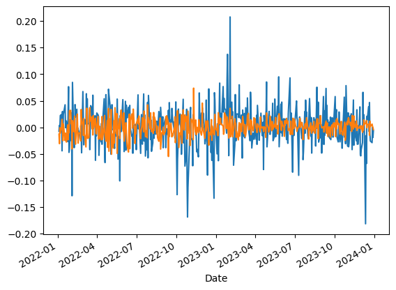
Finally, we plot the hedged portfolio returns alongside the benchmark to visually assess the results.

1hedged_portfolio_returns.plot()
2benchmark_returns.plot()

The results show drastically reduced portfolio returns now that we no longer have such high sensitivity to the benchmark.

On the surface this might seem like a bad idea, but remember: we care about risk adjusted returns (not just returns). We have isolated returns to that of the stocks while neutralizing the returns to that of the benchmark.

Your next steps

Try changing the tickers in the code to analyze a different set of stocks. Observe how the alpha and beta values change with different portfolios. Experiment with different time periods to see how the market conditions affect your analysis.