“The only free lunch in finance is diversification.”

I’ve heard that saying thousands of times. But diversifying a portfolio the right way is not as easy as just putting equal dollar amounts into each stock.

Many investors struggle with creating a balance that enhances returns while minimizing risk.

“Dollar weighting” fall short completely missing the point of diversification: managing risk.

There’s a smarter way to diversify. We can use the same method as Ray Dalio’s Bridgewater Associates.

By reading today's newsletter, get Python code to build a Risk Parity portfolio based on industry constraints.

Let's go!

Build a Risk Parity portfolio with sector constraints

Creating a risk parity portfolio with risk budgets gives us a structured way to balance risk.

This strategy equalizes risk across different asset classes. It aims to enhance returns while reducing volatility by diversifying risk.

In practice, investors define investment goals and select diversified asset classes like equities and bonds. They assess each class's volatility and correlation, setting risk budgets accordingly. Optimization techniques are used to adjust weights, ensuring a balanced risk distribution.

Professionals, like those at Bridgewater Associates, leverage risk parity to optimize risk-adjusted returns. Their portfolios have shown resilience in volatile markets, such as during the 2008 financial crisis.

This strategy offers potential for improved returns and stability, backed by extensive data analysis and modeling.

Let's see how it works with Python.

Imports and set up

Riskfolio does most the heavy lifting of optimization. Import it, pandas, and yFinance.

1import pandas as pd
2import riskfolio as rp
3import yfinance as yf

Define the date range and the list of asset tickers. This allows us to decide which assets and time period we are interested in analyzing.

1start = "2016-01-01"
2end = "2019-12-30"
3
4assets = [
5    "JCI", "TGT", "CMCSA", "CPB", "MO", "APA", "MMC", "JPM", "ZION",
6    "PSA", "BAX", "BMY", "LUV", "PCAR", "TXT", "TMO", "DE", "MSFT",
7    "HPQ", "SEE", "VZ", "CNP", "NI", "T", "BA"
8]
9
10prices = yf.download(assets, start=start, end=end)["Adj Close"]
11returns = prices.pct_change().dropna()

We use yFinance to download the adjusted closing prices for our portfolio and compute returns.

Easy.

Create a portfolio and calculate optimal allocation

Next, we create a portfolio object using the returns. This portfolio will be used to perform optimization and calculate the optimal allocation of assets.

1port = rp.Portfolio(returns=returns)
2
3port.assets_stats(method_mu="hist", method_cov="ledoit")
4port.lowerret = 0.00056488 * 1.5
5
6model = "Classic"
7rm = "MV"
8
9w_rp = port.rp_optimization(model=model, rm=rm)

We calculate the portfolio's expected returns and covariance matrix using historical data and the Ledoit-Wolf shrinkage method. We also set a target return.

Historical data estimates returns, while the Ledoit-Wolf method provides a stable covariance matrix.

We define the optimization model and risk measure to guide portfolio optimization. Using risk parity optimization with the "Classic" model and Mean-Variance ("MV") risk measure, we determine optimal asset allocation.

The optimization calculates asset weights to minimize risk and meet return targets.

Define constraints and re-optimize the portfolio

We create a DataFrame to categorize assets by their industry. This categorization will be used to apply constraints during portfolio optimization.

To avoid creating this mapping manually, check out Financial Modeling Prep data which has an API to get industry data for a list of stocks.

1asset_classes = {
2    "Assets": assets,
3    "Industry": [
4        "Consumer Discretionary", "Consumer Discretionary", "Consumer Discretionary",
5        "Consumer Staples", "Consumer Staples", "Energy", "Financials", "Financials",
6        "Financials", "Financials", "Health Care", "Health Care", "Industrials",
7        "Industrials", "Industrials", "Health Care", "Industrials",
8        "Information Technology", "Information Technology", "Materials",
9        "Telecommunications Services", "Utilities", "Utilities",
10        "Telecommunications Services", "Financials"
11    ]
12}
13
14asset_classes = pd.DataFrame(asset_classes)
15asset_classes = asset_classes.sort_values(by=["Assets"])
16
17constraints = {
18    "Disabled": [False, False, False, False, False],
19    "Type": ["All Assets", "Classes", "Classes", "Classes", "Classes"],
20    "Set": ["", "Industry", "Industry", "Industry", "Industry"],
21    "Position": ["", "Financials", "Utilities", "Industrials", "Consumer Discretionary"],
22    "Sign": ["<=", "<=", "<=", "<=", "<="],
23    "Weight": [0.10, 0.2, 0.2, 0.2, 0.2],
24    "Type Relative": ["", "", "", "", ""],
25    "Relative Set": ["", "", "", "", ""],
26    "Relative": ["", "", "", "", ""],
27    "Factor": ["", "", "", "", ""]
28}
29
30constraints = pd.DataFrame(constraints)
31
32A, B = rp.assets_constraints(constraints, asset_classes)
33
34port.ainequality = A
35port.binequality = B
36
37w_rp = port.rp_optimization(model=model, rm=rm)

There’s a lot here but if you look closely, we’re just creating a DataFrame with Python dictionaries.

Here’s what is happening.

We convert the asset classes into a sorted DataFrame and define constraints for the optimization process, specifying limits on the weight of certain asset classes. This helps ensure the portfolio is diversified across different industries.

We convert the constraints into a DataFrame, which is used to set inequality constraints for the portfolio optimization. We define asset constraints using the specified constraints and asset classes. These constraints are then applied to the portfolio optimization process.

We set the portfolio's inequality constraints using the matrices derived from our constraints. We re-run the portfolio optimization to account for these new constraints.

Visualize the optimal portfolio allocation and risk contribution

Ok, let’s see how we did.

1rp.plot_pie(
2    w=w_rp, 
3    others=0.05,
4    nrow=25,
5    height=6,
6    width=10
7)

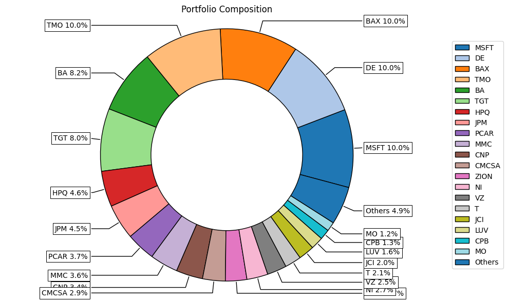
The code generates a pie chart with the optimal weights of each asset.

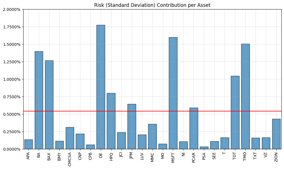
Next, we visualize the risk contribution of each asset in the portfolio. This shows how much each asset contributes to the overall portfolio risk.

1rp.plot_risk_con(
2    w_rp, 
3    cov=port.cov, 
4    returns=port.returns, 
5    height=6,
6    width=10
7)

The risk contribution plot helps us understand which assets contribute most to portfolio risk. It uses the asset weights, covariance matrix, and returns to calculate and visualize risk distribution.

Your next steps

Try modifying the list of assets to include different companies or sectors. You can also adjust the constraints to see how they affect the optimal portfolio allocation. Experiment with different optimization models and risk measures to explore other portfolio strategies.