At the GTC conference, NVIDIA announced that RAPIDS cuML now offers GPU acceleration for scikit-learn.

The cuML accelerator enables significant speedups of up to 50X with no code changes.

This announcement is huge for financial market analysis.

In today's newsletter, you'll run PCA on historical returns of the stocks in the S&P 500. Then, we'll use PCA to analyze potential alpha signals.

All 50X faster.

Let's go!

Accelerate alpha discovery with RAPIDS

PCA isolates the statistical return drivers of a portfolio. These drivers are called “alpha factors” (or just factors) because they create returns that are not explained by a benchmark. (In a previous newsletter issue, you learned how to hedge beta to get exposure to alpha.)

Quants use factors in trading strategies. First, they isolate the components. Then, they buy the stocks with the largest exposure to a factor and sell the stocks with the smallest exposure to a factor. Today, you’ll learn how to do this in Python.

Imports and set up

Start by importing the libraries. sklearn is a package used to build statistical models for data analysis. Note we load the cuML extension using the Jupyter Notebook magic.

1%load_ext cuml.accel
2import yfinance as yf
3import pandas as pd
4import numpy as np
5from sklearn.decomposition import PCA
6import matplotlib.pyplot as plt

Next, use pandas to download a table from Wikipedia. The table contains all the stocks in the S&P 500.

1snp_symbols = pd.read_html("https://en.wikipedia.org/wiki/List_of_S%26P_500_companies")[0].Symbol.tolist()
2symbols = [sym.replace(".", "-") for sym in snp_symbols]
3data = yf.download(symbols, start="2020-01-01", end="2024-12-31")
4portfolio_returns = data['Close'].pct_change().dropna()

Fit the PCA model

sklearn makes it easy to fit a PCA model and get the components.

1pca = PCA(n_components=5)
2pca.fit(portfolio_returns)
3pct = pca.explained_variance_ratio_
4pca_components = pca.components_

The n_components argument tells sklearn how many of the top components to return. Fit the model with the portfolio returns and the algorithm will look for the top three components that explain most of the variance in the returns.

After you fit the model, grab the explained variance and components (remember the underscore).

Visualize the components

If the description of PCA is unclear, these charts should help.

1cum_pct = np.cumsum(pct)
2x = np.arange(1,len(pct)+1,1)
3plt.subplot(1, 2, 1)
4plt.bar(x, pct * 100, align="center")
5plt.title('Contribution (%)')
6plt.xlabel('Component')
7plt.xticks(x)
8plt.xlim([0, 6])
9plt.ylim([0, 100])
10plt.subplot(1, 2, 2)
11plt.plot(x, cum_pct * 100, 'ro-')
12plt.title('Cumulative contribution (%)')
13plt.xlabel('Component')
14plt.xticks(x)
15plt.xlim([0, 6])
16plt.ylim([0, 100])

The result is a chart that looks like this.

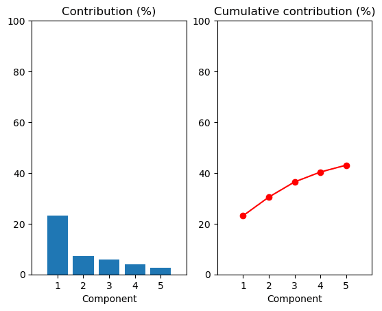
The chart on the left shows the contribution of the top three components toward the total variance. In other words, these components contribute the most to the information in the data. The first component explains about 25% of the variation in the portfolio returns. In stock portfolios, this is usually driven by the overall market movement.

The chart on the right is the cumulative sum of the contribution of each component. It shows the top five components explain about 50% of total portfolio returns.

So what does this actually mean?

Isolate the alpha factors

There are forces that move stock prices that we can't see. These latent factors are picked up through PCA and isolated as the principal components. The overall stock market is usually a strong driver of returns. Macroeconomic forces like interest rates and the pandemic drive returns, too. PCA lets you isolate these statistical factors to get an idea of how much the portfolio’s returns come from these unobserved features.

Let’s take a look.

1X = np.asarray(portfolio_returns)
2factor_returns = X.dot(pca_components.T)
3factor_returns = pd.DataFrame(
4    columns=["f1", "f2", "f3", "f4", "f5"], 
5    index=portfolio_returns.index,
6    data=factor_returns
7)
8factor_returns.head()

First, multiply the portfolio returns by the principal components. The dot function makes sure every return is multiplied by each of the components. the T function transposes the DataFrame. The resulting DataFrame gives you how much of that day’s portfolio return is a result of each of the three factors.

Similar stocks will be driven by similar factors.

Another great way to visualize this is with a scatter plot. Let's look at how the first three factors interact.

1fig = plt.figure()
2ax = fig.add_subplot(111, projection='3d')
3# Use one of the factors for coloring, e.g., f3
4sc = ax.scatter(data[:, 0], data[:, 1], data[:, 2], c=data[:, 2], cmap='viridis')
5ax.set_xlabel('f1')
6ax.set_ylabel('f2')
7ax.set_zlabel('f3')
8plt.colorbar(sc, ax=ax, label='f3')
9plt.show()

The result is a chart that looks like this.

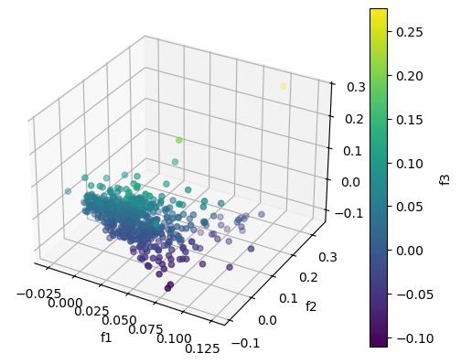
You can see how the stocks are driven by the first three principal components.

This analysis covered the time period during covid. Gold stocks were bid up strongly as a hedge against inflation and uncertainty. You might consider the first factor as a “covid factor” representing uncertainty across the market. Tech stocks crashed as worries of economic health began.

Your next steps

Experiment with different data. Can you find a set that contributes to a higher percentage of explained variance?