Once upon a time, Excel was enough.

You were dealing with a couple thousand rows of data, simple formulas, and a single sheet.

Today, the landscape is much different.

There are millions or billions of rows of data. To complete, you need high powered computing. The models are more complex.

Python and pandas is the solution.

Pandas excels at handling time series data, merging datasets, and performing complex calculations. It streamlines the entire data analysis process.

By reading today's newsletter, you'll learn how to use pandas for better financial market data analysis.

Let's go!

3 examples of using pandas for market data analysis

Pandas is a powerful open-source library for data manipulation and analysis in Python.

It was created in 2008 by Wes McKinney to handle time series data and structured data formats efficiently. Pandas is widely used in financial markets for analyzing investment strategies, historic market prices, and fundamental data.

Pandas introduces key data structures like Series and DataFrames.

It’s great at data manipulation tasks such as merging, reshaping, and cleaning data. Its support for time series data makes it perfect for financial analysis, including date alignment, resampling, and rolling window calculations.

Professionals in finance use pandas for a variety of applications.

They clean and prepare messy financial data, perform time series analysis on stock prices, and optimize portfolios by calculating returns and risk metrics. Pandas also integrates with machine learning libraries for predictive modeling and facilitates effective reporting and visualization of data.

Let's see how it works.

Load historical stock data for a given ticker symbol

We start by loading historical stock data for NVIDIA (ticker symbol "NVDA") from Yahoo Finance. This helps us get the historical prices of the stock to perform further analysis.

1import math
2import pandas as pd
3import yfinance as yf
4import matplotlib.pyplot as plt
5
6data = yf.download("NVDA", start="2023-01-01")

This code uses the yfinance library to download stock data for NVIDIA starting from January 1, 2023. The data is stored in a pandas DataFrame named data. This DataFrame contains various columns such as 'Open', 'High', 'Low', 'Close', 'Volume', and 'Adj Close', which represent different aspects of the stock's daily performance.

Display the first few rows of the data

Next, we display the first few rows of the data to understand its structure and the kind of information it holds.

1data.head()

The head() function in pandas displays the first five rows of the DataFrame by default. This allows us to quickly inspect the data and verify that it has been loaded correctly. We can see the dates as the index and the columns representing different metrics such as opening price, closing price, highest price, lowest price, and volume for each trading day.

Calculate moving averages and other indicators

Now, we calculate the 20-day and 50-day simple moving averages (SMA) of the stock's closing price. We also calculate the historical volatility and the percentile rank of the closing prices.

1data['SMA20'] = data['Close'].rolling(window=20).mean()
2
3data['SMA50'] = data['Close'].rolling(window=50).mean()
4
5data['vol'] = data['Close'].pct_change().rolling(window=21).std() * math.sqrt(252)
6
7data['pct_rank'] = data['Close'].rolling(window=21).rank(pct=True)

We calculate the 20-day and 50-day simple moving averages by using the rolling method with a specified window and then applying the mean function. We compute historical volatility by taking the standard deviation of the daily returns over a 21-day window and then annualizing it using the square root of 252 (number of trading days in a year).

Finally, the percentile rank of the closing prices over a 21-day window is calculated using the rank method with the pct parameter set to True, giving us a value between 0 and 1.

Plot the stock's closing price and moving averages

Next, we plot the stock's closing price along with the 20-day and 50-day simple moving averages to visualize trends and patterns.

1to_plot = ["Close", "SMA20", "SMA50"]
2data[to_plot].plot()

We store the columns to be plotted (closing price, 20-day SMA, and 50-day SMA) in a list named to_plot. Using pandas' plot method, we create a line plot for these columns.

This visual representation helps us see how the stock's price moves relative to its short-term and long-term trends defined by the moving averages.

Plot historical volatility

We then plot the historical volatility of the stock to understand its risk and price fluctuations over time.

1ax = data["Close"].plot()
2data.vol.plot(secondary_y=True, ax=ax)
3plt.show()

This code creates a line plot showing both the closing price and the computed historical volatility.

By plotting these together, we can see how the stock's volatility changes over time and how it correlates with the price movements. Higher volatility indicates higher risk and larger price swings, while lower volatility suggests more stable price behavior.

Plot the percentile rank over time

Finally, we plot the percentile rank of the closing prices to see how the current price compares to its historical range.

1data['pct_rank'].plot()

We use the plot method to visualize the percentile rank of the closing prices. This plot shows how the current price ranks within a specified window of past prices.

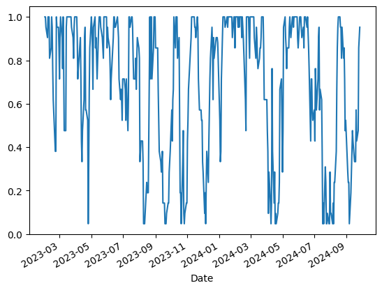
A high percentile rank indicates that the current price is relatively high compared to its historical range, while a low percentile rank suggests that it is relatively low. This can help identify overbought or oversold conditions in the stock.

Your next steps

To deepen your understanding, try changing the stock ticker symbol to analyze a different company's data. You can also experiment with different time windows for the moving averages and volatility calculations to see how these changes affect the results.