In 2006, I got my first hedge fund job (no, not at Renaissance Technologies—RenTec).

I still remember my first day:

A huge room filled with silence, a sea of people, and more screens than a movie theater.

After the usual meet-and-greets and some HR paperwork, I sat down in my chair, ready to conquer the world of trading EUR/USD spot futures.

Things started great.

And ended terribly.

By the end of the day, I'd managed to lose $3,200, which was 32 pips on my 10 lot.

Not quite the entrance I'd envisioned, but there was good news:

It was simulated trading.

As time went by, I discovered that the most successful traders had something in common (and nope, it wasn't their knack for losing fake money):

They used filters to help pinpoint trading signals.

What most algorithmic trading systems get wrong—and RenTec gets right.

Market inefficiencies are hard to find and don't always exist.

That's where filters, like a bandpass filter, come in handy.

Imagine you're at a party with lots of people talking, and you only want to hear people with higher voices (like kids) and lower voices (like some adults) but not the voices in the middle. 

A bandpass filter would only allow the higher and lower voices to reach your ears while blocking the middle ones.

It helps traders focus on specific price movements or trends while ignoring the noisy or random fluctuations in the market.

This makes it easier to identify buying or selling opportunities, leading to better decisions and potentially higher profits.

Unfortunately, most beginners don't use filters

We’re going to change that today.

Imports and set up

Today, you’ll use TA-Lib to create the cycle phases, SciPy to build the bandpass filter, and OpenBB for data.

1from math import pi
2
3from scipy.signal import butter, filtfilt
4import numpy as np
5import talib
6
7import matplotlib.pyplot as plt
8
9from openbb_terminal.sdk import openbb

Use OpenBB to download the EUR/USD price and get the returns.

1data = openbb.forex.load(
2    from_symbol="EUR", 
3    to_symbol="USD", 
4    start_date="2016-01-01", 
5    end_date="2021-12-31"
6)
7
8prices = (
9    data["Adj Close"]
10    .to_frame()
11    .rename(
12        columns={
13            "Adj Close": "close"
14        }
15    )
16)
17
18prices["log_return"] = (
19    prices.close
20    .apply(np.log)
21    .diff(1)
22)

Build the cycle model and filter

The first step is to find the dominant phase of the time series using the Hilbert Transform, then use it to model a cycle inefficiency in the market.

Next is the dominant cycle period which is a signal processing technique that isolates the most significant patterns in prices.

1# Hilbert Transform - Dominant Cycle Phase
2prices["phase"] = talib.HT_DCPHASE(prices.close)
3
4# Convert into a wave using a cycle model
5prices["signal"] = np.sin(prices.phase + pi / 4)
6
7# Use the Hilbert Transform - Dominant Cycle Period
8prices["period"] = talib.HT_DCPERIOD(prices.close)

This code calculates the dominant cycle, a modeled signal from the prices, and the dominant cycle period.

Next, create the bandpass filter.

1def butter_bandpass(data, period, delta=0.5, fs=5):
2    nyq = 0.5 * fs
3
4    # Low cutoff frequency
5    low = 1.0 / (period * (1 + delta))
6    low /= nyq
7
8    # High cutoff frequency
9    high = 1.0 / (period * (1 - delta))
10    high /= nyq
11
12    b, a = butter(2, [low, high], btype="band")
13
14    return filtfilt(b, a, data)
15
16def roll_apply(e):
17    close = prices.close.loc[e.index]
18    period = prices.period.loc[e.index][-1]
19    out = butter_bandpass(close, period)
20    return out[-1]

The Butterworth filter is designed to have a frequency response that is as flat as possible in the passband.

You can use it as a bandpass filter centered around the dominant cycle period.

Pandas cannot create a rolling calculation with two variables, so you need a helper function.

Now it’s time to filter the data and measure the amplitude.

1prices["filtered"] = (
2    prices.dropna()
3    .rolling(window=30)
4    .apply(lambda series: roll_apply(series), raw=False)
5    .iloc[:, 0]
6)
7
8prices["amplitude"] = (
9    prices.
10    filtered
11    .rolling(window=30)
12    .apply(
13        lambda series: series.max() - series.min()
14    )
15)
16
17prices["ema_amplitude"] = (
18    talib
19    .EMA(
20        prices.amplitude,
21        timeperiod=30
22    )
23)

In the first function, you apply the bandpass filter to a rolling window of price data. This only lets the strongest signals found in the price data through.

When the smoothed amplitude is at a peak or valley, the maket is showing signs that the market inefficiency you modeled is present and should be traded.

Analyze the results

Set a signal threshold that you want to use to trigger trades. Then set an amplitude above which indicates the market inefficiency exists and build your positions.

1signal_thresh = 0.75
2amp_thresh = 0.004  # 40 pips
3
4prices["position"] = 0
5prices.loc[
6    (prices.signal >= signal_thresh) & 
7    (prices.amplitude > amp_thresh), "position"
8] = -1
9prices.loc[
10    (prices.signal <= -signal_thresh) &amp; 
11    (prices.amplitude > amp_thresh), "position"
12] = 1

In practice, both the signal and amplitude threshold can (and should) be modeled and optimized.

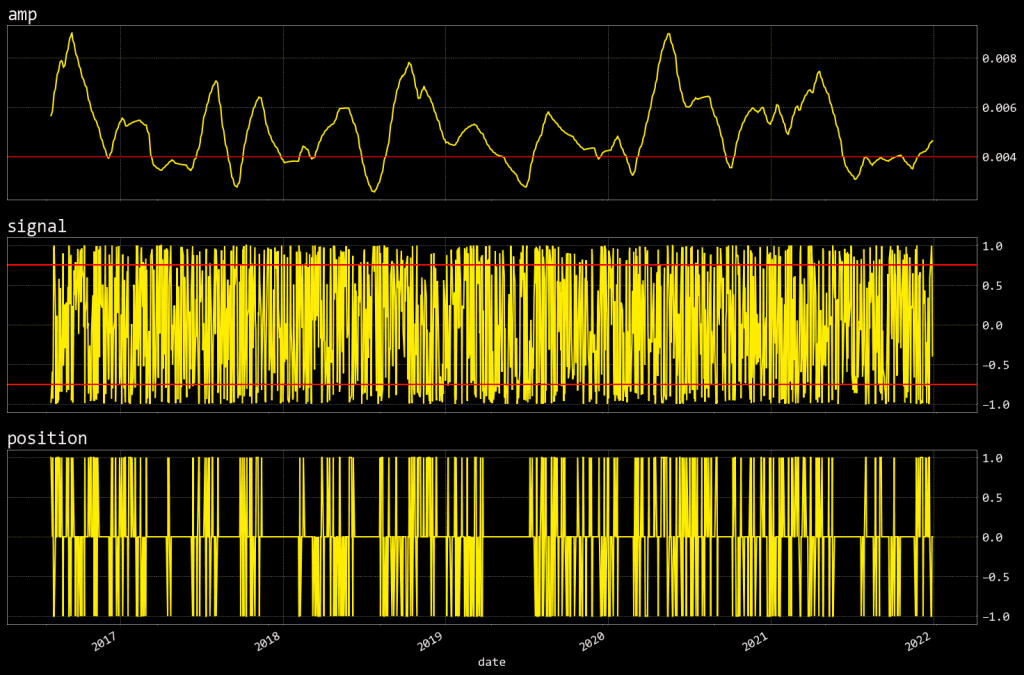
To visualize what’s going on, plot it.

1fig, axes = plt.subplots(
2    nrows=3,
3    figsize=(15, 10),
4    sharex=True
5)
6
7prices.ema_amplitude.plot(
8    ax=axes[0],
9    title="amp"
10)
11axes[0].axhline(
12    amp_thresh,
13    lw=1,
14    c="r"
15)
16prices.signal.plot(
17    ax=axes[1],
18    title="signal"
19)
20axes[1].axhline(
21    signal_thresh,
22    c="r"
23)
24axes[1].axhline(
25    -signal_thresh,
26    c="r"
27)
28prices.position.plot(
29    ax=axes[2],
30    title="position"
31)
32fig.tight_layout()

The top chart is the amplitude of the filtered prices and is used to determine when the market inefficiency exists.

The second chart is the signal which oscillates between -1 and 1. In this example, the signal is a cycle model of market prices.

I use a naive strategy of entering short when the signal exceeds 0.75 and entering long when the signal goes below -0.75.

The last chart shows the position either long (1), short (-1), or flat.

Signal processing techniques are used by the most successful investment firms ever to exist, including RenTec. Now you can build your own price filter to amplify market inefficiencies for more successful trading.