


Quickly store 2,370,886 rows of historic options data with ArcticDB
Over 1,200,000 options contracts trade daily. Storing options data for analysis has become something only professionals can do using sophisticated tools.
One of the professionals recently open sourced their tools for lightening fast data storage and retrieval.
ArcticDB is a DataFrame database that is used in production by the systematic trading company, Man Group.
It’s used for storage, retrieval, and processing petabyte-scale data in DataFrame format.
In today’s newsletter, we’ll use it to store 2,370,886 rows of historic options data.
Quickly store 2,370,886 rows of historic options data
ArcticDB is an embedded, serverless database engine, tailored for integration with pandas and the Python data science ecosystem.
It can efficiently store a 20-year historical record of over 400,000 distinct securities under a single symbol with sub-second retrieval.
In ArcticDB, each symbol is treated as an independent entity without data overlap.
The engine operates independently of any additional infrastructure requiring only a functional Python environment and object storage access.
It uses common object storage solutions such as S3-compatible storage systems and Azure Blob Storage or local storage but can also store data locally in the LMDB format, which we’ll use today.
You can follow along with today’s newsletter with data you can download here.
Ready to get started?
Imports and set up
First, import the libraries we need. We’ll use some base Python modules to import the CSV files.
1import os
2import glob
3import matplotlib.pyplot as plt
4import datetime as dt
5
6import arcticdb as adb
7import pandas as pd
Create a locally hosted LMDB instance in the current directory and set up an ArcticDB library to store the options data.
1arctic = adb.Arctic("lmdb://equity_options")
2lib = arctic.get_library("options", create_if_missing=True)
Now build a helper function that accepts a file path, reads in a CSV file, resets the index, and parses the date strings to pandas Timestamps.
1def read_chains(fl):
2    df = (
3        pd
4        .read_csv(fl)
5        .set_index("date")
6    )
7    df.index = pd.to_datetime(df.index)
8    return df
After you download the sample data, unzip it to the same directory where you’re writing the code.
1files = glob.glob(os.path.join("rut-eod", "*.csv"))
2for fl in files:
3    chains = read_chains(fl)
4    chains.option_expiration = pd.to_datetime(chains.option_expiration)
5    underlyings = chains.symbol.unique()
6    for underlying in underlyings:
7        df = chains[chains.symbol == underlying]
8        adb_sym = f"options/{underlying}"
9        adb_fcn = lib.update if lib.has_symbol(adb_sym) else lib.write
10        adb_fcn(adb_sym, df)
It first retrieves a list of CSV files from the "rut-eod" directory and iterates through them.
For each file, it reads the options chains, converts the 'option_expiration' field to a datetime format, and then processes each unique underlying symbol found in these chains.
The code then determines whether to update or write new data to a storage system based on whether the symbol already exists in the database.
The result is end of day historic options data with 2,370,886 quotes between 2006-07-28 and 2014-09-04.
Using the ArcticDB query builder
We’ll use the powerful QueryBuilder class to retrieve options data for a given as of date and expiration date. We’ll also filter the data based on a range of delta values.
1def read_vol_curve(as_of_date, underlying, expiry, delta_low, delta_high):
2    q = adb.QueryBuilder()
3        filter = (
4            (q["option_expiration"] == expiry) &
5            (
6                (
7                    (q["delta"] >= delta_low) & (q["delta"] <= delta_high)
8                ) | (
9                    (q["delta"] >= -delta_high) & (q["delta"] <= -delta_low)
10                )
11            )
12        )
13    q = (
14        q[filter]
15        .groupby("strike")
16        .agg({"iv": "mean"})
17    )
18    return lib.read(
19        f"options/{underlying}",
20        date_range=(as_of_date, as_of_date),
21        query_builder=q
22    ).data
This function builds a query to filter options that match the expiry and that fall within the given delta range.
It then groups these options by their strike price and calculates the average implied volatility for each group.
Finally, the function returns the aggregated data for the specified underlying asset and as-of date, returning the processed data.
Next, use the same filtering pattern to extract the expiration dates.
1def query_expirations(as_of_date, underlying, dte=30):
2    q = adb.QueryBuilder()
3    filter = (q.option_expiration > as_of_date + dt.timedelta(days=dte))
4    q = q[filter].groupby("option_expiration").agg({"volume": "sum"})
5    return (
6        lib
7        .read(
8            f"options/{underlying}",
9            date_range=(as_of_date, as_of_date),
10            query_builder=q
11        )
12        .data
13        .sort_index()
14        .index
15    )
We retrieve a list of expiration dates with total trading volumes for a given underlying asset. It filters options expiring more than dte days after the specified as_of_date, aggregates the trading volume by expiration date, and then sorts these dates.
Chart the implied volatility curves
We’ll use the stored options data to create a chart of the implied volatility curves on a specified date. These curves are referred to as the implied volatility skew.
First, set some parameters.
1as_of_date = pd.Timestamp("2013-06-03")
2expiry = pd.Timestamp("2013-06-22")
3underlying = "RUT"
4dte = 30
5delta_low = 0.05
6delta_high = 0.50
Then generate the chart.
1expiries = query_expirations(as_of_date, underlying, dte)
2_, ax = plt.subplots(1, 1)
3cmap = plt.get_cmap("rainbow", len(expiries))
4format_kw = {"linewidth": 0.5, "alpha": 0.85}
5for i, expiry in enumerate(expiries):
6    curve = read_vol_curve(
7        as_of_date,
8        underlying,
9        expiry,
10        delta_low,
11        delta_high
12    )
13    (
14        curve
15        .sort_index()
16        .plot(
17            ax=ax,
18            y="iv",
19            label=expiry.strftime("%Y-%m-%d"),
20            grid=True,
21            color=cmap(i),
22            **format_kw
23        )
24    )
25ax.set_ylabel("implied volatility")
26ax.legend(loc="upper right", framealpha=0.7)
The result is a chart of the implied volatility skew across the expiration dates on a given date.
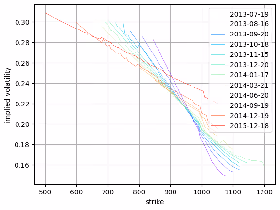
It first retrieves a list of expiration dates and then iterates over these dates, fetching the IV curve for each.
Each curve is plotted on a subplot with a unique color from a rainbow colormap, labeled with its expiration date, and formatted according to specified parameters. The plot is finalized with labels for implied volatility on the y-axis and a legend indicating each expiration date's curve.
Next steps
There are two steps you can take to further the analysis. First, read the documentation for the ArcticDB QueryBuilder which is an important feature of the library. Then, recreate this example and use the other data to further your analysis.