


How to easily improve your Sharpe ratio (in no time)
Systematic risk affects the entire market and impacts the Sharpe ratio. Any trading strategy must consider the impact of systematic risk. While a strategy must involve some risk to make money, systematic risk cannot be diversified away.
So, we need to build a hedge to get rid of it.
By hedging systematic risk, we can better protect our strategies and ultimately outperform the market.
After having taught 1,000+ in my course, I can say with confidence most people do not hedge. Or if they do, it’s ineffective.
By reading today’s newsletter, you’ll see how an effective hedge can improve performance.
Let’s go!
How to easily improve your Sharpe ratio (in no time)
The value of a trading strategy is its ability to deliver good risk-adjusted returns measured by the Sharpe Ratio. In Richard Grinold’s “The Fundamental Law of Active Management,” the Sharpe Ratio can be thought of in two components: skill and breadth. Skill is measured by the Information Coefficient (IC). Breadth is measured by the number of independent trades.
Factor investing is what made me stand out at JPMorgan.
— PyQuant News 🐍 (@pyquantnews) February 27, 2024
But it took me years to master the information coefficient.
In 1 minute, I'll teach you the 10 things you need to know (that took me 1 year to learn).
Let's go: pic.twitter.com/2CsrtI7xKv
Higher breadth, when combined with skill, increases the potential for good risk-adjusted returns.
By hedging systematic risk, we can increase the number of independent bets and improve breadth. This increase in breadth leads to better performance and higher returns. That’s why managing systematic risk is important for optimizing the Sharpe Ratio.
Let’s see how it works.
Imports and set up
We’ll use yFinance for asset data and statsmodels for simple regression. Let’s import the libraries.
In this analysis, we’ll use three financial stocks and three energy stocks. You can replace these with your own portfolio.
The result is two plots. The first shows the historic stock price. The second shows the correlation matrix.

The average pairwise correlation across the six assets in our portfolio is 0.628. This is quite high and restricts our ability to make independent bets.
Hedging systematic sector risk
Now let’s run the analysis again with ETFs that represent the financial sector, energy sector, and overall market.
This code repeats the process we did before including the ETFs representing our sectors. Next, we do some DataFrame manipulation to isolate the stock returns.
Note the two DataFrames, residuals_market and residuals, which are copies of stock_returns but filled with zeros. We’ll use these next. In this code, we begin to isolate the specific returns of stocks by removing the effects of broader market movements and sector influences.
The sector return and the market return are themselves highly correlated. As such, you cannot do a multivariate regression due to multicollinearity.
To hedge against both the market and a given security’s sector, you first estimate the market beta residuals and then calculate the sector beta on those residuals.
The function ols_residual calculates the residuals from an ordinary least squares (OLS) regression of y on **x. This**represents the portion of y not explained by x. The variables sector_1_excess and sector_2_excess store the excess returns of two sectors over the market returns.
The loops iterate over stocks in each sector. First, we remove the market influence from each stock’s returns and then remove the sector influence. This double regression isolates the idiosyncratic returns of each stock to make sure the residuals represent independent bets.
Finally, we can plot the residuals and test the correlation of the hedged portfolio.
The result is two plots. The first shows the historic residuals. The second shows the correlation matrix.

The average pairwise correlation across the six assets in our portfolio is 0.024. The sector hedge brought down the correlation between our bets to close to zero.
Calculating effective breadth
We’ll use the “semi-generalized fundamental law of active management” to calculate breadth. This ideas is from David Buckle’s work, “How to calculate breadth: An evolution of the fundamental law of active portfolio management,” published in the Journal of Asset Management in 2003.
The key takeaway for us is a closed-form calculation of effective breadth based on the correlation between bets. The result is a chart that shows us the effective breadth for each level of forecasted correlation.
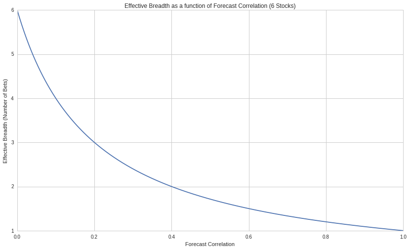
We see that at a correlation 0.628, we are effectively making only approximately one bet. When we add the sector hedge, we get close to zero correlation, and in this case the number of bets equals the number of assets, six.