


How to backtest 2,000,000 simulations for the best exits
If you're using backtesting to optimize parameters to maximize PnL,
— PyQuant News 🐍 (@pyquantnews) August 15, 2023
you're going to lose money.
Your backtest is a framework to test:
• Statistical significance of your strategy
• Sensitivity to parameter changes
• Impact of transaction costs
Not to overfit to noise. pic.twitter.com/gp3RJWLA0g
Backtests are not a way to brute force optimize parameters to maximize a performance metric.
Doing that leads to overfitting and losses.
But optimization does play an important part in building trading strategies.
Today, we’ll see how.
How to backtest 2,000,000 simulations for the best exits
A backtest is a simulation of market dynamics which are used to test how trading strategies might perform behaved.
The problem is that the markets are noisy and difficult to model.
So when running backtests, optimized models often fit to noise, instead of market inefficiencies. When applying the optimized parameters to previously unseen data, the model falls apart (along with your portfolio).
All parameters of a strategy affect the result but only a few determine entry and exit dependent on the market price. These are the parameters that should be optimized.
For example, is a 1% trailing stop better than a $1 stop loss?
We’ll use the cutting-edge backtesting framework vectorbt to optimize the entry and exit type for a momentum strategy.
Strap on your seatbelt.
Let’s go!
Imports and set up
Given the power of what we’re about to do, there are very few imports required.
We’ll set some variables for the analysis.
vectorbt has built in data download capability using yFinance but it takes a bit of manipulation to get it right.
The code downloads historical and is then concatenated into a single DataFrame. We use the vectorbt range_split method to evenly split the market data into separate lookbacks.
We then initialize an empty dictionary called split_ohlcv to store the split data. Finally, we iterate through each symbol’s data and split it into smaller time windows and store the split data in the split_ohlcv dictionary.
Build the momentum strategy
Our strategy selects the top 3 stocks every split based on their mean return. The strategy equally allocates across the stocks at the beginning of the period, and exits at the end.
The code calculates the momentum of each stock symbol based on the percentage change of their closing prices. It then sorts these values within each split and selects the top 3 stocks with the highest momentum.
Finally, it extracts the prices of the selected stocks using their indices and stores them in selected_open, selected_high, selected_low, and selected_close, respectively.
Test the order types
There’s a lot of code here. But we’re essentially creating the exit positions based on the different order types.
The code creates an empty DataFrame with the same shape as selected_open and sets the first row to True which is our entry point.
It then calculates three types of exit signals: stop-loss (sl_exits), trailing stop (ts_exits), and take-profit (tp_exits).
The levels of these DataFrames are renamed for clarity, and the last row of each DataFrame is set to True to ensure an exit at the end of the split.
Finally, we concatenate the exit signals into a single DataFrame called exits, with a new index level to differentiate between the three exit strategies.
Run and analyze the backtest
Now that we have our data, entries, and exits, we can run the optimization and analyze the results.
The result shows a histogram of total returns based on each stop type.
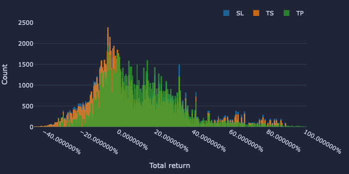
We can see that the trailing stop seems to have more negative returns while the take-profit has more positive returns. Let’s take a different look.
The result is a box plot with the order types.
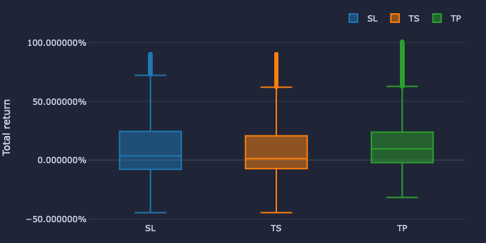
We can use the box plot to confirm that the take-profit order type outperforms the two others. Let’s quantify it further.
You’ll see that the mean total return for the take-profit order type is 12.3% while that for the other two are below 10%.
Next steps
vectorbt is an advanced library suitable for walk-forward analysis and optimization.
The next step is to get get the code running on your machine and learn more about the framework by reading the documentation.If you’ve been a reader of this newsletter for a while, or a student of Getting Started With Python for Quant Finance, you’ll recognize this statement: