


Build state-of-the-art portfolios with machine learning
Portfolio optimization usually requires an estimate of the future returns of the assets in the portfolio. This is hard because we can’t see into the future.
Risk parity is a strategy that uses risk to find the allocations of an investment portfolio.
— PyQuant News 🐍 (@pyquantnews) October 29, 2022
It allocates money to stocks based on a target risk level - usually volatility.
Instead of equal *dollar* weights, risk parity portfolios have equal *risk* weights. pic.twitter.com/AsvGeRqG4C
Traditional risk parity uses a quadratic optimizer
A cutting edge technique called Hierarchical Risk Parity (HRP) uses graph theory and machine learning to build a hierarchical structure of the investments.
By the end of today’s newsletter, you’ll be able to create your own HRP-based portfolio among 25 sector-based ETFs.
Are you ready?
Build state-of-the-art portfolios with machine learning
HRP was introduced by Marcos Lopez de Prado in a 2016 paper. HRP applies graph theory and machine learning to build a diversified portfolio based on the covariance matrix.
HRP is unlike traditional portfolio optimization methods. It can create an optimized portfolio when the covariance matrix is ill-degenerated or singular. This is impossible for quadratic optimizers.
Research has shown HRP to deliver lower out-of-sample variance than traditional optimization methods.
Let’s get started!
Imports and set up
We’ll use the excellent RiskFolio-Lib to build our HRP portfolio and OpenBB for market data.
We’ll use market data from 25 sector-based ETFs to construct our portfolio.
This code uses OpenBB to download the market data as a DataFrame and generate the daily returns for each ETF.
Build the optimal portfolio
We can plot the dendrogram to visualize which ETFs are clustered together.
The result is the following image.

The plot visualizes the hierarchical clustering of assets based on their historical return correlations. It illustrates how clusters of assets are merged at each hierarchical level and can give us insight into the correlation structure within a portfolio. The method takes asset returns and a clustering method to compute and plot the dendrogram.
Building the optimal portfolio based on the hierarchy is one line of code.
The codependence parameter is set to "pearson" to use the Pearson correlation to measure the relationships between asset returns. The risk measure is set to "MV" for minimum variance which minimizes the portfolio's overall volatility.
Additional parameters like linkage, max_k, and leaf_order are specified to fine-tune the clustering and dendrogram construction process.
The result is a pandas Series with the optimal weight for each of the assets.
Visualize the results
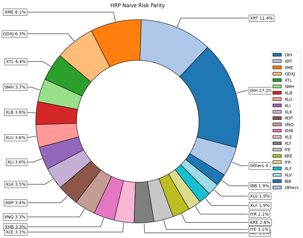
RiskFolio-Lib makes it easy to visualize the results of the optimization.
This code generates a pie chart which with the weights of each asset.
We can also visualize the risk contribution of each asset.
The risk contribution of each asset in a portfolio quantifies how much individual assets contribute to the total risk, considering both their own volatility and their correlation with other assets. We can see the highest risk contribution is from OIH which is an oil ETF.
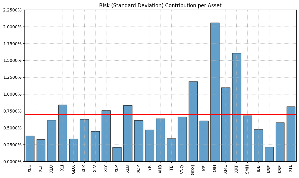
Risk contribution is important for identifying assets that disproportionately increase portfolio risk.
Next steps
We only scratched the surface of HRP. As a next step, add the assets in your portfolio and optimize it for a risk measure other than variance. You can try “MAD”, “CVaR”, or “VaR.” Check the documentation for details.