


Backtest powerful intraday trading strategies
Multi-timeframe (MTF) analysis lets traders build powerful intraday trading strategies.
It does this by analyzing asset prices during different timeframes throughout the trading day.
The problem is most people get MTF wrong.
It requires a vector-based backtest to speed up the operations making it easy to introduce look-ahead bias.
When a backtest introduces look-ahead bias, it will overstate performance.
So how do we do MTF analysis “the right way?”
By reading today’s newsletter, you’ll be able to use VectorBT Pro (VBT) to to MTF the right way.
Backtest powerful intraday trading strategies
Many vector-based backtesters assume events take place at the same timestamp as the data provided by the exchange.
This is typically the opening time of a bar.
VBT takes a different approach.
It assumes the timing of most events is unknown and occurs between the opening (best-case) and closing (worst-case) times of a bar.
To do this, VBT uses a set of features designed to resample data in the most sensitive way, without looking into the future.
Sound complicated?
It’s only a few lines of Python code. Let’s see how it works!
Imports and set up
Using the latest version of VBT, the star-import (*) loads all the relevant libraries for us. (Don’t worry, it won’t pollute your namespace.)
Many vector-based backtesters assume events take place at the same timestamp as the data provided by the exchange.
This is typically the opening time of a bar.
VBT takes a different approach.
It assumes the timing of most events is unknown and occurs between the opening (best-case) and closing (worst-case) times of a bar.
To do this, VBT uses a set of features designed to resample data in the most sensitive way, without looking into the future.
Sound complicated?
It’s only a few lines of Python code. Let’s see how it works!
Grab the data of a higher frequency for your favorite asset. We'll use hourly TSLA.
Multi-timeframe indicators
Instruct VBT to calculate the fast and slow SMA indicators across multiple timeframes.
Under the hood, data is first resampled to the target timeframe. Then, the TA-Lib indicator is applied only to non-missing values. Finally, the result is realigned back to the original timeframe in a way that eliminates the possibility of look-ahead bias.
VBT makes it easy to visualize the results.

We can see the line corresponding to the highest frequency is smooth, whereas the line representing the lowest frequency appears stepped since the indicator values are updated less frequently.
Build a unified portfolio
Next, we'll set up a portfolio that goes long whenever the fast SMA crosses above the slow SMA and go short when the opposite occurs, across each timeframe.
Since hourly signals occur more frequently than daily signals, we'll allocate less capital to more frequent signals.
We'll allocate 5% of the equity to hourly signals, 10% to 4-hour signals, and 20% to daily signals.
We'll begin with a cash balance of $10,000, shared across all timeframes. Additionally, we'll implement a 20% trailing stop loss (TSL).
Plot the cumulative return for each timeframe and compare these to the cumulative return of the entire portfolio.
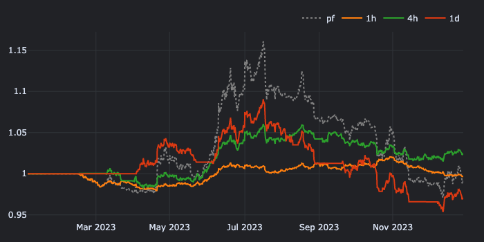
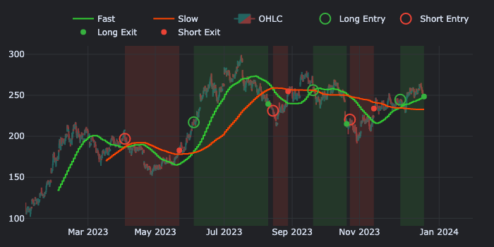
To dive deeper into one of the timeframes, we can plot the indicators alongside the executed trade signals.
Here, we can observe that the majority of positions on the daily timeframe were closed out by the TSL.
Timeframe product
Since our MTF indicators share the same index, we can combine one timeframe with another. Lets generate signals from the crossover of two timeframes and identify the pair of timeframes that yield the highest expectancy.
I looks like the 1 hour fast MA and 4 hour slow MA achieve the highest expectancy of a profitable trade.
Next steps
Timeframe is yet another parameter of your strategy that can be tweaked. For example, you can go to uncharted territory and test more unconventional timeframes like "1h 30min" to discover potentially novel insights. Similar to other parameters, timeframes should also undergo cross-validation.
However, unlike regular parameters, timeframes should be regarded as a distinct dimension that provides a unique perspective on your strategy.