The 1 mistake beginner options traders make that cost them money

In 2005, I traded my first complex options position.

I just got my margin account open and level 3 options trading approved.

Don’t make any mistakes!

I remember the feeling:

Endless possibilities, huge potential, and certainty the market would go my way.

And it did! In a really big way.

Only I put the trade on in the wrong direction (I sold a straddle when I should’ve bought one).

Ouch.

After getting over the shock of seeing $9,800 vaporized in one trading day from my mistake, I decided to seriously learn about trading.

I studied the math, learned Python, and started to analyze options correctly.

But even after all my hard work, I was still making one big mistake:

I was using the wrong options pricing model.

The 1 mistake beginner options traders make that cost them money (and how to avoid it)

An American option is a type of financial contract.

It gives the owner the right to buy or sell an underlying asset at a specified price on or before a specified date.

Unlike European options, which can only be exercised on the expiration date, American options can be exercised at any time before or on the expiration date. To price a European option, you can use a closed-form model like the Black-Scholes framework.

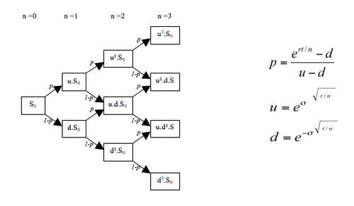
To price an American option, you need a numerical method called the Binomial options pricing model.

This method divides the time to expiration into a series of equally spaced intervals, creating a tree-like structure with nodes representing the possible prices of the underlying asset.

By calculating the option’s value at each node, we can find the option’s price today while accounting for the opportunity of early exercise.

Setup and import

Because you’re using a numerical solution, the only import you need is NumPy.

import numpy as np

Build the function

You can construct the valuation model in a single function.

def american_option_pricer(spot, strike, rate, vol, expiry, steps, option_type):
    # Calculate the time interval and the up and down factors
    dt = expiry / steps
    u = np.exp(vol * np.sqrt(dt))
    d = 1 / u

    # Calculate the risk-neutral probability
    p = (np.exp(rate * dt) - d) / (u - d)

    # Create the binomial price tree
    price_tree = np.zeros((steps + 1, steps + 1))
    for i in range(steps + 1):
        price_tree[i, -1] = spot * (u ** (steps - i)) * (d**i)

    # Calculate the option value at each node
    option_tree = np.zeros_like(price_tree)
    if option_type.lower() == "call":
        option_tree[:, -1] = np.maximum(price_tree[:, -1] - strike, 0)
    elif option_type.lower() == "put":
        option_tree[:, -1] = np.maximum(strike - price_tree[:, -1], 0)
    else:
        raise ValueError("Option type must be either 'call' or 'put'.")

    # Traverse the tree backward to find the option price today
    for t in range(steps - 1, -1, -1):
        for i in range(t + 1):
            exercise = 0
            if option_type.lower() == "call":
                exercise = price_tree[i, t] - strike
            elif option_type.lower() == "put":
                exercise = strike - price_tree[i, t]

            hold = np.exp(-rate * dt) * (
                p * option_tree[i, t + 1] + (1 - p) * option_tree[i + 1, t + 1]
            )
            option_tree[i, t] = np.maximum(exercise, hold)

    return option_tree[0, 0]

These are the steps:

1. Calculate the time interval (dt) and the up (u) and down (d) factors based on the volatility and time interval.

2. Compute the risk-neutral probability p using the interest rate, up, and down factors.

3. Create the binomial price tree, filling it with the possible prices of the underlying asset at each time step.

4. Calculate the option value at the last time step (the expiration date) using the price tree.

5. Traverse the tree backward, comparing the value of exercising the option with the value of holding it (update the option tree with the maximum of these two values).

6. The estimated option price is the value at the root of the option tree (i.e., option_tree[0, 0]).

Now use it.

option_price = american_option_pricer(
    spot=55.0,
    strike=50.0,
    rate=0.05,
    vol=0.3,
    expiry=1.0,
    steps=100,
    option_type="call",
)

This returns the estimated price of a call option.

I spent 6 months pricing American-style options with the Black-Scholes model wondering what was going wrong. So if you’re just getting started, use the right model!